Download
1 / 27
270 likes | 376 Views
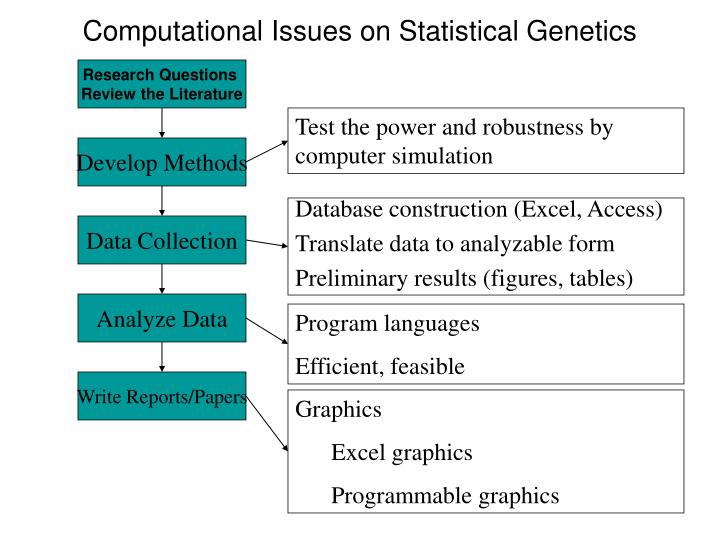
Computational Issues on Statistical Genetics. Research Question s Review the Literature. Test the power and robustness by c omputer simulation. Develop Method s. Database construction (Excel, Access) Translate d ata to analyzable form Preliminary results (figures, tables).

E N D
Computational Issues on Statistical Genetics Research Questions Review the Literature Test the power and robustness by computer simulation Develop Methods Database construction (Excel, Access) Translate data to analyzable form Preliminary results (figures, tables) Data Collection Analyze Data Program languages Efficient, feasible Write Reports/Papers • Graphics • Excel graphics • Programmable graphics
Program Languages • Fortran, C, C++ • Matrix language: MATLAB, S-Plus, R, SAS IML • Symbolic Calculation: Mathematika,Maple,Matlab • Interface Programming: dotnet, C#, Visual Basic • SAS, SPSS, BMDP • Database: Access, Excel, SQL, SAS, Oracle • MACRO • Excel, Access, PowerPoint, Word • Editor: WinEdt • SAS Macro
Two Point Analysis in F2Fully Informative Markers (codominant) BB Bb bb AA Obs n22 n21 n20 Freq ¼(1-r)2½r(1-r)¼r2 Recom. 0 1 2 Aa Obs n12 n11 n10 Freq ½r(1-r) ½(1-r)2+½r2½r(1-r) Recom. 1 2r2/[(1-r)2+r2] 1 aa Obs n02 n01 n00 Freq ¼r2½r(1-r) ¼(1-r)2 Recom. 2 1 0
EM algorithm to estimate the recombination fraction r: • Given r(0), For t=0,1, 2,… • Do While abs[r(t+1)-r(t)]>1.e-8 • E-step: Calculate (t) = r(t)2/[(1-r(t))2+r(t)2] (expected the number of recombination events for the double heterozygote AaBb) • M-step: r(t+1)= 1/(2n)[2(n20+n02)+(n21+n12+n10+n01)+2(t)n11]
Two Point Analysis in F2Fully Informative Markers (codominant) Input: Result: BB Bb bb AA Aa aa n r0 (t) = r(t)2/[(1-r(t))2+r(t)2] r(t+1)= 1/(2n)[2(n20+n02)+(n21+n12+n10+n01)+2(t)n11]
Two Point Analysis in F2Fully Informative Markers (codominant) Matlab program to estimate recombinant r function r=rEstF2(n22,n21,n20,n12,n11,n10,n02,n01,n00) n=n22+n21+n20+n12+n11+n10+n02+n01+n00; r=0.2; r1=-1; while (abs(r1-r)>1.e-8) r1=r; %E-step phi=r^2/((1-r)^2+r^2); %M step r=1/(2*n)*(2*(n20+n02)+(n21+n12+n10+n01)+2*phi*n11); end
Log-likelihood ratio test statistic Two alternative hypotheses H0: r = 0.5 vs. H1: r 0.5 Likelihood value under H1 L1(r|nij) = n!/(n22!...n00!) [¼(1-r)2]n22+n00[¼r2]n20+n02[½r(1-r)]n21+n12+n10+n01[½(1-r)2+½r2]n11 Likelihood value under H0 L0(r=0.5|nij) = n!/(n22!...n00!) [¼(1-0.5)2]n22+n00[¼0.52]n20+n02[½0.5(1-0.5)]n21+n12+n10+n01[½(1-0.5)2+½0.52]n11 LOD = log10[L1(r|nij)/L0(r=0.5|nij)] = {(n22+n00)2[log10(1-r)-log10(1-0.5)+…} = 6.08 > critical LOD=3
Two Point Analysis in F2Fully Informative Markers (codominant) Matlab program to calculate log likelihood test score (LOD) function LOD=calcLOD_F2(r,n22,n21,n20,n12,n11,n10,n02,n01,n00) %%log likelihood under H1 LOD=(n22+n00)*log10((1-r)^2/4)... +(n20+n02)*log10(r^2/4)... +(n21+n12+n10+n01)*log10(r*(1-r)/2)... +n11*log10((1-r)^2/2+r^2/2); %%log likelihood under H0 r=0.5; LOD0=(n22+n00)*log10((1-r)^2/4)... +(n20+n02)*log10(r^2/4)... +(n21+n12+n10+n01)*log10(r*(1-r)/2)... +n11*log10((1-r)^2/2+r^2/2); LOD=LOD-LOD0;
Two Point Analysis in F2Partial Informative Markers (codominant X dominant) BB Bb bb AA Obs n22 n21 n20 Freq ¼(1-r)2 ½r(1-r)¼r2 Recom. 0 1 2 Aa Obs n12 n11 n10 Freq ½r(1-r) ½(1-r)2+½r2½r(1-r) Recom. 1 2r2/[(1-r)2+r2] 1 aa Obs n02 n01 n00 Freq ¼r2½r(1-r) ¼(1-r)2 Recom. 2 1 0
Two Point Analysis in F2Partial Informative Markers (codominant X dominant) B_ bb AA Obs n2_ =n22+n21 n20 Freq ¼(1-r)2+½r(1-r) ¼r2 Recom. C1= ½r(1-r)/[¼(1-r)2+½r(1-r)] 2 Aa Obs n1_ =n12+n11 n10 Freq ½r(1-r)+½(1-r)2+½r2½r(1-r) Recom. C2=[½r(1-r) +r2]/[½r(1-r)+½(1-r)2+½r2] 1 aa Obs n0_ =n02+n01 n00 Freq ¼r2+½r(1-r) ¼(1-r)2 Recom. C3=[2* ¼r2+½r(1-r)]/[¼r2+½r(1-r)] 0 Estimate of r=(c1* n2_ +c2* n1_ +c3* n0_+2* n20 + n00)/(2n)
Two Point Analysis in F2Partial Informative Markers (codominant X dominant) E-Step C1= ½r(1-r)/[¼(1-r)2+½r(1-r)] C2=[½r(1-r) +r2]/[½r(1-r)+½(1-r)2+½r2] C3=[2* ¼r2+½r(1-r)]/[¼r2+½r(1-r)] M-Step r=(c1* n2_ +c2* n1_ +c3* n0_+2* n20 + n00)/(2n)
Two Point Analysis in F2Partial Informative Markers (codominant X dominant) Input: Result: B_ bb AA Aa aa n r0
Two Point Analysis in F2Partial Informative Markers (co dominant X dominant) Matlab program to estimate recombinant r function r=rEstF2CoXdomin(n2_,n1_,n0_,n20,n10,n00) n=n2_+n1_+n0_+n20+n10+n00; r=0.2;r1=-1; while(abs(r1-r)>1.e-8) r1=r; %E-step c1= 1/2*r*(1-r)/[1/4*(1-r)^2+ 1/2*r*(1-r)]; c2=[1/2*r*(1-r)+r^2]/[1/2*r*(1-r)+1/2*(1-r)^2+1/2*r^2]; c3=[2*1/4*r^2+1/2*r*(1-r)]/[1/4*r^2+1/2*r*(1-r)]; %M-step r=(c1*n2_+c2* n1_ +c3* n0_+2* n20 + n00)/(2*n); end
Two Point Analysis in F2Partial Informative Markers (co dominant X dominant) Matlab program to calculate log likelihood test score (LOD) function LOD=calcLOD_F2CoXdomin(r, n2_,n1_,n0_,n20,n10,n00) %%log likelihood under H1 LOD=log([1/4*(1-r)^2+ 1/2*r*(1-r)])*n2_ ... +log([1/2*r*(1-r)+1/2*(1-r)^2+1/2*r^2])*n1_ ... +log([1/4*r^2+1/2*r*(1-r)])*n0_ ... +log(r^2/4)*n20+log(r*(1-r)/2)*n10+log((1-r)^2/4)*n00; %%log likelihood under H0 r=0.5; LOD0=log([1/4*(1-r)^2+ 1/2*r*(1-r)])*n2_ ... +log([1/2*r*(1-r)+1/2*(1-r)^2+1/2*r^2])*n1_ ... +log([1/4*r^2+1/2*r*(1-r)])*n0_ ... +log(r^2/4)*n20+log(r*(1-r)/2)*n10+log((1-r)^2/4)*n00; LOD=LOD-LOD0; LOD=LOD/log(10);
Two Point Analysis in F2Partial Informative Markers (dominant) BB Bb bb AA Obs n22 n21 n20 Freq ¼(1-r)2½r(1-r)¼r2 Recom. 0 1 2 Aa Obs n12 n11 n10 Freq ½r(1-r) ½(1-r)2+½r2½r(1-r) Recom. 1 2r2/[(1-r)2+r2] 1 aa Obs n02 n01 n00 Freq ¼r2½r(1-r) ¼(1-r)2 Recom. 2 1 0
Two Point Analysis in F2Partial Informative Markers (dominant) B_ bb A_ Obs n1 =n22+n21 +n12 +n11 n2=n20 +n10 Freq ¼(1-r)2 +r(1-r)+½(1-r)2+½r2¼r2 Recom. c1 c2 aa Obs n3=n02+n01 n4=n00 Freq ¼r2 +½r(1-r) ¼(1-r)2 Recom. C2= (2(¼r2 )+½r(1-r))0 /(¼r2 +½r(1-r)) where C1=[r2+r(1-r)]/[ ¼(1-r)2 +r(1-r)+½(1-r)2+½r2],expected number of recombinant gametes Estimate of r=(c1* n1 +c2* n2 +c2* n3)/(2n)
Two Point Analysis in F2Fully Informative Markers (codominant) Input: Result: B_ bb A_ aa n r0 C1=[r2+r(1-r)]/[ ¼(1-r)2 +r(1-r)+½(1-r)2+½r2], C2= (2(¼r2 )+½r(1-r)) /(¼r2 +½r(1-r)) Estimate of r=(c1* n1 +c2* n2 +c2* n3)/(2n)
Two Point Analysis in F2Partial Informative Markers (dominant) Matlab program to estimate recombinant r function r=rEstF2Partial(n1,n2,n3,n4) n=n1+n2+n3+n4; r=0.2;r1=-1; while (abs(r1-r)>1.e-8) r1=r; %E-step c1=(r^2+r*(1-r))/((1-r)^2/4+r*(1-r)+(1-r)^2/2+r^2/2); c2=(r^2/2+r*(1-r)/2)/(r^2/4+r*(1-r)/2); %M-step r=1/(2*n)*(c1*n1+c2*n2+c2*n3); end
Log-likelihood ratio test statisticPartial Informative Markers (dominant) Two alternative hypotheses H0: r = 0.5 vs. H1: r 0.5 Likelihood value under H1 L1(r|nij) = n!/(n1!...n4!) [3/4(1-r)2 +r(1-r)+½r2]n1[¼r2 +½r(1-r)]n2+n3[¼(1-r)2]n4 Likelihood value under H0 L0(r=0.5|nij) = n!/(n1!...n4!) [3/4(1-.5)2 +.5(1-.5)+½.52]n1[¼.52 +½.5(1-.5)]n2+n3[¼(1-.5)2]n4 LOD = log10[L1(r|nij)/L0(r=0.5|nij)] = 3.17 > critical LOD=3
Two Point Analysis in F2Partial Informative Markers (dominant) Matlab program to calculate log likelihood test score (LOD) function LOD=calcLOD_F2Partial(r,n1,n2,n3,n4) %%log likelihood under H1 LOD=(n1)*log10((1-r)^2*3/4+r^2/2+r*(1-r))... +(n2+n3)*log10(r^2/4+r*(1-r)/2)... +(n4)*log10((1-r)^2/4); %%log likelihood under H0 r=0.5; LOD0=(n1)*log10((1-r)^2*3/4+r^2/2+r*(1-r))... +(n2+n3)*log10(r^2/4+r*(1-r)/2)... +(n4)*log10((1-r)^2/4); LOD=LOD-LOD0;
chrom1 chrom2 chrom3 chrom4 RG218 RG437 RG104 RG472 13.0 7.7 8.1 RZ262 RG348 RG544 8.6 19.2 5.3 13.2 RG190 RG246 RZ329 12.6 RG171 6.9 16.1 22.2 RZ892 RG908 9.8 13.7 K5 RG157 RG91 4.8 2.8 RG100 3.2 U10 RG449 4.7 27.4 RG532 17.5 RG191 16.1 RZ318 RG788 15.3 6.3 RZ678 8.4 W1 RZ565 15.5 RG173 16.8 29.3 Pall 41.6 RZ675 Amy1B 15.0 21.4 RZ58 RZ574 3.8 RZ276 10.2 RG163 CDO686 37.1 3.3 RG146 8.8 RZ284 28.2 Amy1A/C RZ590 34.3 15.6 12.8 2.7 RG345 RZ394 RG214 2.5 RG95 8.4 18.5 12.2 RG381 pRD10A RG143 23.5 RG654 5.1 2.5 5.9 RZ19 RZ403 10.0 RG620 8.2 RG256 RG690 5.0 5.4 RG179 28.6 13.2 RZ730 13.1 RZ213 CDO337 1.9 RZ123 RZ337A 33.1 22.5 RZ801 RZ448 RG520 15.0 2.6 RG810 RZ519 RG331 32.1 9.2 Pgi -1 7.1 CDO87 9.2 RG910 17.9 RG418A
Three Point Analysis in Backcross Summarized the data as
Rice Data Marker RG472 denoted by A, RG246 by B, K5 by C
Multilocus likelihood – determination of a most likely gene order • Consider three markers A, B, C, with no particular order assumed. • A triply heterozygous F1 ABC/abc backcrossed to a pure parent abc/abc Genotype ABC or abc ABc or abC Abc or aBC AbC or aBc Obs. n00 =69 n01=12 n10=16 n11=3 Frequency under Order A-B-C (1-rAB)(1- rBC) (1-rAB) rBC rAB(1- rBC) rAB rBC Order A-C-B (1-rAC)(1- rBC) rAC rBC rAC(1-rBC)(1-rAC)rBC Order B-A-C (1-rAB)(1- rAC) (1-rAB) rAC rABrAC rAB(1-rAC) rAB = the recombination fraction between A and B= (n10 + n11)/n=0.19 rBC = the recombination fraction between B and C=(n01 + n11)/n=0.15 rAC = the recombination fraction between A and C=(n01 + n10)/n=0.28
What order is the mostly likely? LABC (1-rAB)n00+n01 (1-rBC)n00+n10 (rAB)n10+n11 (rBC)n01+n11 LACB (1-rAC)n00+n11 (1-rBC)n00+n10 (rAC)n01+n10 (rBC)n01+n11 LBAC (1-rAB)n00+n01 (1-rAC)n00+n11 (rAB)n10+n11 (rAC)n01+n10 Log(LABC) = -90.8932 Loo(LACB) = -101.5662 Log(LBAC) = -107.9176 According to the maximum likelihood principle, the linkage order that gives the maximum likelihood for a data set is the best linkage order supported by the data. the best linkage order A B C 20cM 15cM
DATA Genotype ABC or abc ABc or abC Abc or aBC AbC or aBc Obs. n00 =69 n01=12 n10=16 n11=3 Result: rAB = =0.19 rBC = =0.15 rAC = =0.28 dAB=1/4*ln[(1+2 rAB)/(1-2 rAB)]=20 dBC=1/4*ln[(1+2 rBC)/(1-2 rBC)]=15 Log(LABC) = -90.8932 Loo(LACB) = -101.5662 Log(LBAC) = -107.9176 the best linkage order A B C 20cM 15cM