Download
1 / 39
390 likes | 585 Views
Computational Genetics Lecture 1. Background Readings : Chapter 2&3 of An introduction to Genetics, Griffiths et al. 2000, Seventh Edition (CS/Fishbach/Other libraries).

E N D
Computational GeneticsLecture 1 Background Readings: Chapter 2&3 of An introduction to Genetics, Griffiths et al. 2000, Seventh Edition (CS/Fishbach/Other libraries). This class has been edited from several sources. Primarily from Terry Speed’s homepage at Stanford and the Technion course “Introduction to Genetics”. Changes made by Dan Geiger. .
Human Genome Most human cells contain 46 chromosomes: • 2 sex chromosomes (X,Y): XY – in males. XX – in females. • 22 pairs of chromosomes, named autosomes.
Genetic Information • Gene – basic unit of genetic information. They determine the inherited characters. • Genome – the collection of genetic information. • Chromosomes – storage units of genes.
egg sperm zygote gametes Sexual Reproduction Meiosis
The Double Helix Source: Alberts et al
Chromosome Logical Structure Marker – Genes, SNP, Tandem repeats. Locus – location of markers. Allele – one variant form of a marker. Locus1 Possible Alleles: A1,A2 Locus2 Possible Alleles: B1,B2,B3
Alleles - the ABO locus example O is recessive to A. A is dominant over O. A and B are codominant. Multiple alleles: A,B,O. Trait = Character = Phenotype
X-linked • b- dominant allele. Namely, (b,b), (b,w) is Black. • w - recessive allele. Namely, only (w,w) is White. This is an example of an X-linked trait/character. For males b alone is Black and w alone is white. There is no homolog gene on the Y chromose. genotype phenotype
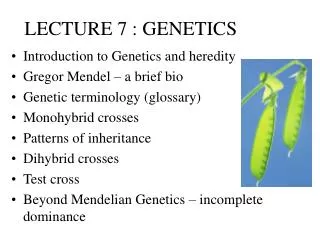
Mendel’s Work Modern genetics began with Mendel’s experiments on garden peas (Although, the ramification of his work were not realized during his life time). He studied seven contrasting pairs of characters, including: The form of ripe seeds: round, wrinkled The color of the seed albumen: yellow, green The length of the stem: long, short Mendel Gregor. 1866. Experiments on Plant Hybridization. Transactions of the Brünn Natural History Society.
Mendel’s first law Characters are controlled by pairs of genes which separate during the formation of the reproductive cells (meiosis) A a a A
P: AA X aa F1: Aa F1 X F1 Aa X Aa test cross Aa X aa Gametes: A a A AA Aa a Aa aa Gametes: A a a Aa aa ~ ~ Phenotype: 1A : 1 a F2: 1 AA : 2 Aa : 1 aa ~ ~ Phenotype A a
Mendel’s second law When two or more pairs of genes segregate simultaneously, they do so independently. A a; B b A B Ab a B ab PAB= PA PB PAb=PA Pb PaB=Pa PB Pab=Pa Pb
Recombination Phenomenon(Happens during Meiosis) Recombination Haplotype Male or female The recombination fraction Between two loci on the same chromosome Is the probability that they end up in regions Of different colors תאי מין: ביצית, או זרע
O A2/A2 A A1/A1 1 2 A A2/A2 A A1/A2 3 4 A | O A2 | A2 A O A1 A2 O O A2 A2 O O A1 A2 Recombinant O A1/A2 5 Example: ABO, AK1 on Chromosome 9 Phase inferred Hardy-Weinberg law of population genetics permits calculation of genotype frequencies from allele frequencies P(a)= frequency of “a” in the population P(ab) =2P(a)P(b) Hardy-Weinberg equilibrium corresponds to a random union of two gamets, called zygote.
O A2/A2 A A1/A1 1 2 A A2/A2 A A1/A2 3 4 A | O A2 | A2 A O A1 A2 O O A2 A2 O O A1 A2 Recombinant O A1/A2 5 Example: ABO, AK1 on Chromosome 9 Phase inferred Recombination fraction is 12/100 in males and 20/100 in females. One centi-morgan means one recombination every 100 meiosis. One centi-morgan corresponds to approx 1M nucleotides (with large variance) depending on location and sex.
Maximum Likelihood Principle What is the probability of data for this pedigree, assuming a recessive mutation ? What is the probability of data for this pedigree, assuming a dominant mutation ? Maximum likelihood principle: Choose the model that maximizes the probability of the data.
Linkage Equilibrium • Linkage Equilibrium =haplotype frequency is the product of the underlying allele’s frequencies: independence. • Exceptions occur for tightly linked loci.
One locus: founder probabilities Founders are individuals whose parents are not in the pedigree. They may of may not be typed (namely, their genotype measured). Either way, we need to assign probabilities to their actual or possible genotypes. This is usually done by assuming Hardy-Weinberg equilibrium (H-W). If the frequency of D is .01, then H-W says: pr(Dd ) = 2x.01x.99 Genotypes of founder couples are (usually) treated as independent. pr(pop Dd , mom dd ) = (2x.01x.99)x(.99)2 D d 1 1 2 D d dd
One locus: transmission probabilities Children get their genes from their parents’ genes, independently, according to Mendel’s laws; also independently for different children. D d D d 1 2 d d 3 pr(kid 3 dd | pop 1 Dd & mom 2 Dd ) = 1/2 x 1/2
One locus: transmission probabilities - II D d D d 1 2 4 3 5 d d D d D D pr(3 dd & 4 Dd & 5 DD | 1 Dd & 2 Dd ) = (1/2 x 1/2)x(2 x 1/2 x 1/2) x (1/2 x 1/2). The factor 2 comes from summing over the two mutually exclusive and equiprobable ways 4 can get a D and a d.
One locus: penetrance probabilities Pedigree analyses usually suppose that, given the genotype at all loci, and in some cases age and sex, the chance of having a particular phenotype depends only on genotype at one locus, and is independent of all other factors: genotypes at other loci, environment, genotypes and phenotypes of relatives, etc. Complete penetrance: pr(affected | DD ) = 1 Incomplete penetrance) pr(affected | DD ) = .8 DD DD
One locus: penetrance - II Age and sex-dependent penetrance (liability classes) pr( affected | DD , male, 45 y.o. ) = .6 D D(45)
One locus: putting it all together 2 1 D d D d 3 5 4 D D D d d d Assume penetrances pr(affected | dd ) = .1, pr(affected | Dd ) = .3 pr(affected | DD ) = .8, and that allele D has frequency .01. The probability of data for this pedigree assuming penetrances of 1=0.1 and 2=0.3 is the product: (2 x .01 x .99 x .7) x (2 x .01 x .99 x .3) x (1/2 x 1/2 x .9) x (2 x 1/2 x 1/2 x .7) x (1/2 x 1/2 x .8) This is a function of the penetrances. By the maximum likelihood principle, the values for 1 and 1 that maximize this probability are the ML estimates.
Linkage & Recombination Tutorial #2 by Ma’ayan Fishelson .
Crossing Over • Sometimes in meiosis, homologous chromosomes exchange parts in a process called crossing-over. • New combinations are obtained, called the crossover products.
Recombination During Meiosis Recombinantgametes
Linkage • 2 genes on separate chromosomes assort independently at meiosis. • 2 genes far apart on the same chromosome can also assort independently at meiosis. • 2 genes close together on the same chromosome pair do not assort independently at meiosis. • A recombination frequency << 50% between 2 genes shows that they are linked.
A A B B a a b b A a B b a a b b A a b b A a B b 1 2 3 4 5 6 Two Loci Inheritance Recombinant
The farther apart U & V are the greater the chance that a crossing over would occur between them the greater the chance of recombination between them. Linkage Maps • Let U and V be 2 genes on the same chromosome. • In every meiosis, chromatids cross over at random along the chromosome. • If the chromatids cross over between U & V, then a recombinant is produced.
Recombination Fraction • The recombination fraction between two loci • is the percentage of times a recombination • occurs between the two loci. • is a monotone, nonlinear function of the • physical distance separating between the loci • on the chromosome.
Centimorgan (cM) • 1 cM (or 1 genetic map unit, m.u.) is the distance between genes for which the recombination frequency is 1%.
Interference • Crossovers in adjacent chromosome regions are usually not independent. This interaction is called interference. • A crossover in one region usually decreases the probability of a crossover in an adjacent region.
Building Genetic Maps • At first: only genes with variant alleles producing detectably different phenotypes were used as markers for mapping. • Problem: the chromosomal intervals between the genes were too large the resolution of the maps wasn’t high enough. • Solution: use of molecular markers (a site of heterozygosity for some type of silent DNA variation not associated with any measurable phenotypic DNA variation).
Linkage Mapping by Recombination in Humans. • Problems: • It’s impossible to make controlled crosses in humans. • Human progenies are rather small. • The human genome is immense. The distances between genes are large on average.
Lod Score for Linkage Testing by Pedigrees The results of many identical matings arecombined to get a more reliable estimate of the recombination fraction. • Calculate the probabilities of obtaining a set of results in a family on the basis of (a) independent assortment and (b) a specific degree of linkage. • Calculate the Lod score = log(b/a). A Lod score of 3 is considered convincing support for a specific recombination fraction.