Download
1 / 21
210 likes | 211 Views
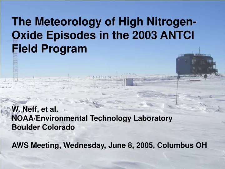
The Meteorology of High Nitrogen- Oxide Episodes in the 2003 ANTCI Field Program. W. Neff, et al. NOAA/Environmental Technology Laboratory Boulder Colorado AWS Meeting, Wednesday, June 8, 2005, Columbus OH. Past observations of high surface NO concentrations at the South Pole.

E N D
The Meteorology of High Nitrogen- Oxide Episodes in the 2003 ANTCI Field Program W. Neff, et al. NOAA/Environmental Technology Laboratory Boulder Colorado AWS Meeting, Wednesday, June 8, 2005, Columbus OH
Past observations of high surface NO concentrations at the South Pole • Nitrogen Oxide (NO) concentrations, larger than expected, were found in field programs in December 1998 and November-December 2000. Davis et al. suggested one explanation lay in shallow mixing layers and nonlinear chemistry, but direct confirming measurements were not available. • To address this issue we developed a sodar specifically focused on the lowest layers of the atmosphere to support the ANTCI 2003 field program.
The Experiment: Atmospheric Research Observatory 22-m Tower Sodar Balloon System Surface System
Wind Speed Note that subcritical Richardson number occurs below the height of maximum echoes
An example: NO Profile The half-hour averaged data marks the strong echoes at the top of the layer where the facsimile record shows what appear to Kelvin-Helmholtz instabilities.
Result: Higher NO with echo-layers less than 50 m in depth ?
Depth Scaling comparisons with sodar data and surface NO First results from 2000, using spectral scaling, appeared to overestimate depths (Oncley et al). We then tested the relationship from Pollard et al (1973), derived for the oceanic mixed layer and used previously with some success at the South Pole (Neff, 1980): H=1.2 u* (fNB) -1/2 1. Depth essentially varies linearly with surface stress 2. Weak dependence on stability 3. Assumes a steady solution (obtained at inertial periods of 12 hours).
Depth Scaling results compared with sodar data Predicted with two different sources of ΔT Analysis of the period from JD 347 to 363 with full supporting data gave us confidence that the sodar could characterize the first portion of the field program that began about JD 320.
Results from the second half of the 2003 experimental period behaved similarly to past experiments. However, the period in late November was quite unusual with persistently high NO concentrations, even with deeper mixing layers. Period prior to JD340 shows sustained high NO values: What was different?
Higher NO prior to the vortex breakup than after for the same mixing layer depth Implication from 2003 field program: Delays in the spring time breakup of the polar vortex affects surface chemistry
A result: Higher NO prior to breakup of the “ozone hole” for the same mixing layer depth Ozone-depleted region located over source region during light, downslope wind regimes
Questions: • Was the NO chemistry different? • Was the meteorology unusual? • What supporting meteorological observations were available during the “early” period? • Did the sodar analysis miss something? • Are the characteristics of the periods different? • What does the AWS network say about the regionality of the episodes?
Henry and Nico lie 100 km grid north and east, respectively of the South Pole. Nico was out of order during 2003. Twice daily (~0830 UTC and ~2100 UTC) GPS rawinsondes produce “relatively” high resolution profiles.
Example from 2003 using AWS’s Henry and SP: Examining JD 327 in more detail
Day 327: NO=321 pptv NO=761 pptv
Day 332: NO=500 pptv
Day 334: NO=683 pptv
Wind speed differences: SP, Nico, Henry (1998) South Pole v. Nico Henry v. Nico NO (pptv)
Summary: • Rawinsondes and the Sodar data give some measure of insight in the NO episodes. • NICO may be a ideal upstream site for analysis of potential stagnation conditions upwind of the South Pole (but only one case so far). • Are other measurements possible on AWS such as ∆T? More AWS?
Future work: • Continued work with the ANTCI program to understand synoptic influences on surface chemistry. • Examination of the role of Indian Ocean warming on tropospheric trends over Antarctica • Results to be presented at • IAMAS, August 2005 (Neff and Hoerling)