Download
1 / 55
550 likes | 674 Views
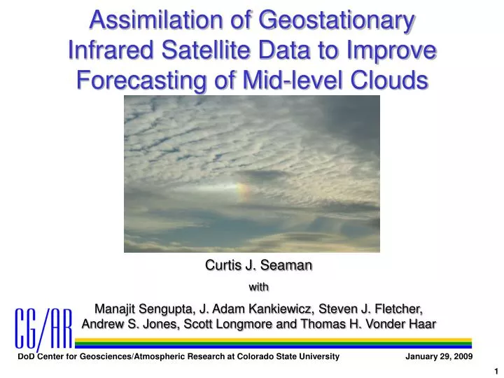
Assimilation of Geostationary Infrared Satellite Data to Improve Forecasting of Mid-level Clouds. Curtis J. Seaman with Manajit Sengupta, J. Adam Kankiewicz, Steven J. Fletcher, Andrew S. Jones, Scott Longmore and Thomas H. Vonder Haar.

E N D
Assimilation of Geostationary Infrared Satellite Data to Improve Forecasting of Mid-level Clouds Curtis J. Seaman with Manajit Sengupta, J. Adam Kankiewicz, Steven J. Fletcher, Andrew S. Jones, Scott Longmore and Thomas H. Vonder Haar
Assimilation of Geostationary Infrared Satellite Data to Improve Forecasting of Mid-level Clouds Objectives: Improve forecasting of mid-level clouds Assimilate GOES Imager and Sounder data into the 4-DVAR RAMDAS Compare results with observations from CLEX-9 Investigate the assimilation of cloudy-scene radiances into a cloud-free model state Photo: Curtis Seaman
Outline Introduction to mid-level clouds and DoD relevance RAMDAS and GOES Assimilation of GOES Imager (ch. 3 & 4) Assimilation of GOES Sounder (ch. 7 & 11) Assimilation of water vapor channels only Variation of decorrelation lengths and variance (background error covariance) Conclusions and Future Work
DoD Relevance Mid-level Clouds have a significant impact on DoD operations Altocumulus and altostratus clouds cover 20-25% of the globe Form between 2 km and 7 km MSL (mission critical altitudes) Obscure surface targets, pilot visibility Interfere with infrared (IR) and laser based communication systems Source of supercooled liquid droplets (aircraft icing) and turbulence These ground Unmanned Aircraft Systems (UAS) Difficult to forecast
Difficult Clouds to Forecast • Operation Desert Storm prompted CLEX • During CLEX-9, eight clouds were observed by aircraft, none were forecast by models we used • RAMS, Eta, RUC, NOGAPS, MM5, ECMWF • CloudNet also found European regional and global models under-forecast mid-level clouds Image: Illingworth et al. (2007)
Quit Being So Difficult • Field studies show that altocumulus clouds are generally: • Less than 1 km thick • Have vertical velocities less than 2 m s-1 • Contain both liquid droplets and ice crystals • Operational models typically: • Have coarse vertical resolution in the mid-troposphere (~500 m or more) • Have a tough time accurately simulating vertical velocity and cloud microphysics • Have poor moisture information (radiosonde dry-bias)
2 Nov 2001 Altocumulus from CLEX-9 • RAMS run with 100 m vertical resolution initialized with Eta 40 km reanalysis • Peak RH of 85% too low to form cloud • Radiosonde dry bias? • Will assimilation of IR water vapor radiances help?
Satellite DA in Cloudy Areas? • Operational forecast centers typically assimilate only cloud-free radiances • Ease, computational cost • McNally and Vespirini (1995); Garand and Hallé (1997); Ruggiero et al. (1999); McNally et al. (2000); Raymond et al. (2004); Fan and Tilley (2005) • Clouds cover 51-67% of the globe • ISCCP, CLAVR, Warren et al. (1986,1988) • Area of recent research • Vukicevic et al. (2006) • Marecal and Mahfouf (2002), Bauer et al. (2006), Weng et al. (2007) Image: NASA
Regional Atmospheric Modeling Data Assimilation System (RAMDAS) • Mesoscale 4-DVAR assimilation system designed to assimilate clear and cloudy scene VIS, IR satellite data • Forward model: RAMS • Observational operator: VISIROO • SHDOM, OPTRAN, Deeter and Evans (1998) • Developed for GOES (Imager & Sounder) • Full adjoints for VISIROO and RAMS • Includes RAMS microphysics, but not convective parameterizations
start end No Yes Regional Atmospheric Modeling Data Assimilation System (RAMDAS) Compute gradient of cost function and decide whether it is small enough yet Satellite radiance over assimilation time window Forward NWP model Forward Radiative Transfer to compute radiance from model output Update initial condition using propagated gradient of cost function. Reverse or adjoint of radiative transfer to compute adjoints Reverse or adjoint of NWP model to compute adjoints Generate forecast Greenwald et al. (2002) Zupanski et al. (2005)
The 2 Nov 2001 Altocumulus Image: RAP@UCAR
Imager Ch. 1 VIS 0.63 mm Sounder Ch. 19 VIS 0.70 mm Ch. 4 window 10.7 mm Ch. 7 window 12.0 mm Ch. 3 vapor 6.7 mm Ch. 11 vapor 7.0 mm
Experiment Set-Up 75 x 75 (6 km horiz.) x 84 (stretched-z vert.) grid centered on North Platte, NE Lateral boundaries masked to 50 x 50 x 84 to ignore boundary condition errors RAMS initialized with 00 UTC FNL (GDAS) reanalysis data 11 UTC output used to initialize RAMDAS 1145 UTC GOES observations assimilated Control Variables: p qil u,v,w rice rsnow rtotal pressure (pert. Exner function) ice-liquid potential temperature winds ice water mixing ratio snow water mixing ratio total water mixing ratio
Initial Forward Model Run Initial model is poor, but we’ll use it (and get valuable results)
Experiment #1: Imager only GOES Imager channels 3 (6.7 mm) & 4 (10.7 mm)
Experiment #1: Imager only GOES Imager channels 3 (6.7 mm) & 4 (10.7 mm) Before Assimilation After Assimilation Observed Tb
Experiment #1: Imager only GOES Imager channels 3 (6.7 mm) & 4 (10.7 mm) Before assimilation After assimilation Observed sounding = dashed Model sounding = solid
Experiment #1: Imager only GOES Imager channels 3 (6.7 mm) & 4 (10.7 mm)
Experiment #1: Imager only GOES Imager channels 3 (6.7 mm) & 4 (10.7 mm)
Experiment #1: Imager only GOES Imager channels 3 (6.7 mm) & 4 (10.7 mm)
Experiment #1: Imager only GOES Imager channels 3 (6.7 mm) & 4 (10.7 mm) Surface wind (before) Surface wind (after)
Experiment #1: Imager only GOES Imager channels 3 (6.7 mm) & 4 (10.7 mm)
Experiment #2: Sounder only GOES Sounder channels 7 (12.02 mm) & 11 (7.02 mm)
Experiment #2: Sounder only GOES Sounder channels 7 (12.02 mm) & 11 (7.02 mm) Before Assimilation After Assimilation Observed Tb
Experiment #2: Sounder only GOES Sounder channels 7 (12.02 mm) & 11 (7.02 mm) Before assimilation After assimilation
Experiment #2: Sounder only GOES Sounder channels 7 (12.02 mm) & 11 (7.02 mm)
Experiment #2: Sounder only GOES Sounder channels 7 (12.02 mm) & 11 (7.02 mm)
Experiment #2: Sounder only GOES Sounder channels 7 (12.02 mm) & 11 (7.02 mm)
Experiment #2: Sounder only GOES Sounder channels 7 (12.02 mm) & 11 (7.02 mm) Surface wind (before) Surface wind (after)
Experiment #2: Sounder only GOES Sounder channels 7 (12.02 mm) & 11 (7.02 mm)
Experiment #3: water vapor only GOES Imager ch 3 (6.7 mm) & Sounder ch 11 (7.02 mm)
Experiment #3: water vapor only GOES Imager ch 3 (6.7 mm) & Sounder ch 11 (7.02 mm) Before Assimilation After Assimilation Observed Tb
Experiment #3: water vapor only GOES Imager ch 3 (6.7 mm) & Sounder ch 11 (7.02 mm) Before assimilation After assimilation
Experiment #3: water vapor only GOES Imager ch 3 (6.7 mm) & Sounder ch 11 (7.02 mm)
Experiment #3: water vapor only GOES Imager ch 3 (6.7 mm) & Sounder ch 11 (7.02 mm)
Experiment #3: water vapor only GOES Imager ch 3 (6.7 mm) & Sounder ch 11 (7.02 mm)
Experiment #3: water vapor only GOES Imager ch 3 (6.7 mm) & Sounder ch 11 (7.02 mm) Surface wind (before) Surface wind (after)
Experiment #3: water vapor only GOES Imager ch 3 (6.7 mm) & Sounder ch 11 (7.02 mm)
Decorrelation Lengths Background error covariance matrix, B, in RAMDAS based on decorrelation length and variance Assumed values of decorrelation length for each control variable shown Decorrelation lengths and variances doubled and halved
Decorrelation Lengths Increasing (decreasing) decorrelation length increases (decreases) impact of observations Variance (not shown) had little effect Note: dashed lines correspond to soundings based on default values of decorrelation length
Mid-level Cloud Decorrelation Lengths Doubled Imager Experiment Sounder Experiment
Summary • GOES Imager experiment • Cooled the surface, increased upper-tropospheric humidity • Increased fog • No closer to producing mid-level cloud • GOES Sounder experiment • Produced subsidence inversion • Cooled, humidified atmosphere near 2 km AGL • Some surface cooling • No mid-level cloud, but closer to producing one • Water Vapor-only experiment • Produced weaker subsidence inversion near 2 km AGL • Almost no effect on the surface • Similar to GOES Sounder results otherwise
Conclusions • The assimilation modifies the model state where the observations are sensitive to model variables • When no cloud is present in the model, the adjoint calculates sensitivities based on having no cloud • In the GOES Imager case, ch. 4 is most sensitive to surface temperature in the absence of cloud, ch. 3 is most sensitive to upper-tropospheric humidity • GOES Sounder ch. 7 & 11 are more sensitive to low- to mid- troposphere temperature and humidity • Significant innovations achieved with only one observation time • Biggest changes to temperature, dew point and winds • Many implications for other cases • Clouds in multiple layers • Clouds over snow • Clouds of different scales
Back to the Future • More channels, more observation times • More case studies • CLEX-9, CLEX-10 • Ideal decorrelation lengths • Add constraints • Surface temperature • Additional cloud information • Log-normal distributions (Fletcher and Zupanski 2007)
Model Resolution Models typically have course vertical resolution in the mid-troposphere RUC layers are set at 2 K (qv) in mid-troposphere Fleishauer et al. (2002) showed qv varied by less than 2 K within cloud ~500 m resolution not uncommon in other models
What We Have Learned about Mid-level Mixed-Phase Clouds Generating Cells ~ 1-1.5 km in Length Optically Opaque Mixed-Phase Region (~300-500 m deep) Precipitating Ice Region (~.2-2.5 km deep) Supercooled Liquid = = Ice
What We Have Learned about Mid-level Mixed-Phase Clouds Icing and Turbulence Region! Supercooled Liquid = = Ice
AVN model Forecast Model Microphysics Models typically assume the colder it is, the more ice there is