Download
1 / 18
180 likes | 187 Views
Using data assimilation to improve estimates of C cycling. Mathew Williams School of GeoScience, University of Edinburgh. Terrestrial Carbon Dynamics. DATA. DATA +Direct observation, good error estimates -Gaps, incomplete coverage. MODEL-DATA FUSION. MODELS. MODELS

E N D
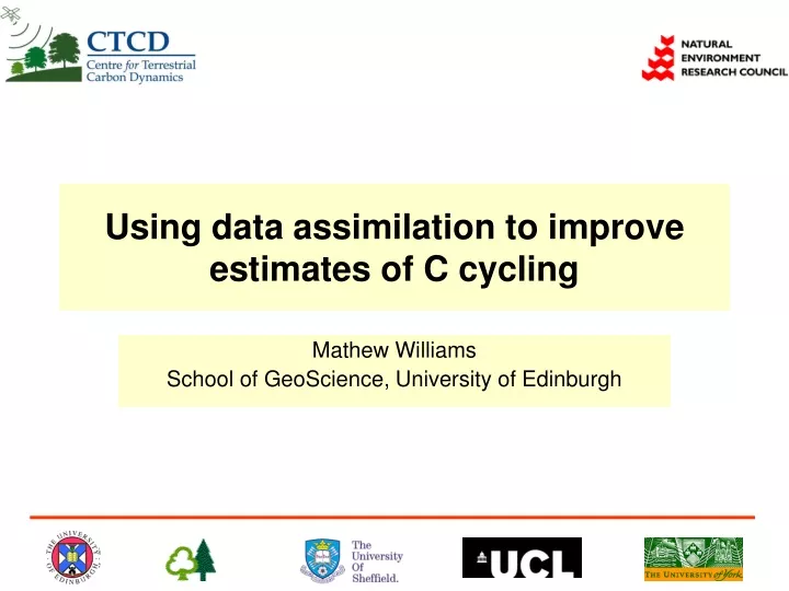
Using data assimilation to improve estimates of C cycling Mathew Williams School of GeoScience, University of Edinburgh
Terrestrial Carbon Dynamics DATA DATA +Direct observation, good error estimates -Gaps, incomplete coverage MODEL-DATA FUSION MODELS MODELS +Knowledge of system evolution -Poor error estimates
Eddy fluxes Leaf chamber Soil chamber Litter traps CO2 ATMOSPHERE Carbon flow Photosynthesis Autotrophic Respiration Heterotrophic respiration Leaves Litterfall Stems Translocation Litter Roots Soil biota Decomposition Soil organic matter
A prediction-correction system Time update “predict” Measurement update “correct” Initial conditions
ψ is the state vector j counts from 1 to N, where N denotes ensemble number k denotes time step, M is the model operator or transition matrix dq is the stochastic forcing representing model errors from a distribution with mean zero and covariance Q error statistics can be represented approximately using an appropriate ensemble of model states Ensemble Kalman Filter: Prediction Generate an ensemble of observations from a distribution mean = measured value, covariance = estimated measurement error. dj = d +ejd = observations e = drawn from a distribution of zero mean and covariance equal to the estimated measurement error
ψf = forecast state vector ψa = analysed estimate generated by the correction of the forecast Ensemble Kalman Filter: Update H is the observation operator, a matrix that relates the model state vector to the data, so that the true model state is related to the true observations by dt= H ψ t Ke is the Kalman filter gain matrix, that determines the weighting applied to the correction
Rtotal & Net Ecosystem Exchange of CO2 Af Lf Cfoliage Rh Ra Ar Lr GPP Croot Clitter D 6 model pools 10 model fluxes 9 rate constants 10 data time series Aw Lw Cwood CSOM/CWD C = carbon pools A = allocation L = litter fall R = respiration (auto- & heterotrophic) Temperature controlled
Setting up the analysis • The state vector contains the 6 pools and 10 fluxes • The analysis updates the state vector, while parameters are unchanging during the simulation • Test adequacy of the analysis by checking whether NEP estimates are unbiased
Setting up the analysis II • Initial conditions and model parameters • Set bounds and run multiple analyses • Data uncertainties • Based on instrumental characteristics, and comparison of replicated samples. • Model uncertainies • Harder to ascertain, sensitivity analyses required
Multiple flux constraints Ra = 0.47 GPP Williams et al. 2005
Af = 0.31 Aw=0.25 Ar=0.43 Turnover Leaf = 1 yr Roots = 1.1 yr Wood = 1323 yr Litter = 0.1 yr SOM/CWD =1033 yr Williams et al. 2005
Parameter uncertainty • Vary nominal parameters and initial conditions ±20% • Generate 400 sets of parameters and IC’s, and then generate analyses • Accept all with unbiased estimates of NEP (N=189) • The mean of the NEE analyses over three years for unbiased models (-421±17 gC m-2) was little different to the nominal analysis (419±29 g C m-2)
Discussion • Analysis produces unbiased estimates of NEP • Autocorrelations in the residuals indicate the errors are not white • Litterfall models over simplified • Relative short time series and aggrading system • Next steps: assimilating EO products, and long time series inventories
Heterotrophic and autotrophic respiration Fraction of total respiration Ra = 42% Rh = 58%