Download
1 / 31
310 likes | 383 Views
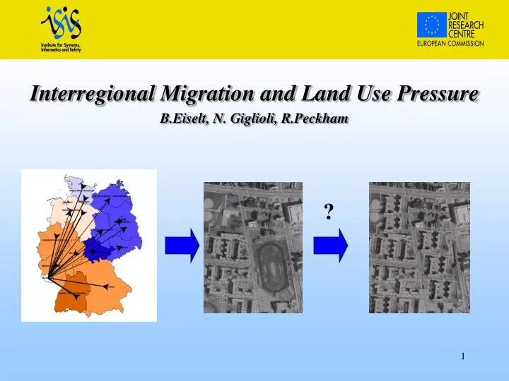
Interregional Migration and Land Use Pressure B.Eiselt, N. Giglioli, R.Peckham. ?. Acknowledgement. Based mainly on work carried out in the project: Lot 4: “Spatial Analysis of interregional migration in correlation with other socio-economic statistics” Performed by JRC for EUROSTAT

E N D
Interregional Migration and Land Use Pressure B.Eiselt, N. Giglioli, R.Peckham ?
Acknowledgement Based mainly on work carried out in the project: Lot 4: “Spatial Analysis of interregional migration in correlation with other socio-economic statistics” Performed by JRC for EUROSTAT from July 1998-July 1999 by: B.Eiselt, N. Giglioli, R.Peckham, A. Saltelli, T.Sorensen
Outline Interregional migration modeling: Data and Software Spatial Interaction models Cluster analysis Modeling Results GIS based Visualization tool Speculation on land use pressure: Link to urban expansion Ideas for modeling Index for pressure
Data and Software • Databases: • GISCO - admin. boundaries (NUTS1 & 2) • REGIO - socio-economic data + flow matrices Software: • SPSS 8.0 for statistical analysis • ARC-VIEW GIS (standard in E.C.)
Spatial Interaction Models Description Exploratory analysis Estimation of the models Parameters interpretation Simulation
Models description • The General Spatial InteractionModelhas the form • where: • i - parameters which characterise the propensity of each origin to generate flows; • j -parameters which characterise the attractiveness of each destination; • is a distance deterrence effect.
Models description • Four types: • Double Constrained - exploring attractive properties of destinations and repulsive properties of origins • Origin Constrained, and Destination Constrained - finding explanatory variables • Unconstrained Model • - finding explanatory variables, and simulating
Models description To apply the ordinary least squares fitting we make a Logarithmic transformation of the model in a way that the the error is Normal distributed
Correlation analysis Analysis of correlation (Germany example) Variables OUT_total IN_total GDP UNEMP OUT_total 1 0.89 -0.67 0.96 IN_total 1 0.93 -0.57 GDP 1 -0.57 UNEMP 1
Cluster analysis • Grouping together regions displaying similar properties, • - based on the values of: • total inflow divided by population, • total outflow divided by population, • GDP per inhabitant, • unemployment rate ( % of total workforce). • These variables are relative and are hence not influenced by the population size of the regions.
Models Estimation - Model choice: - Method: Least Square and stepwise regression method - Indicator Goodness of Fit: R2 adjusted
Statistics ! Kurtosis ? Poisson distribution ? NORMALISED ?? ALL OK ! Normal distribution ? Assumptions ? Central Limit Theorem ? Skewness ?
Models Estimation Model estimated for Germany 1991: Adj -R2 = 0.74 logYij = 1.767+0.934logGDPi+0logUnpi+ +0.829logGDPj+0.739logUnpj-1.156logdij Note: the unemployment of origin is not significant
Simulation ? Model fit (1991) R2 = 74%; Forecast (1993) R2 = 65.6%
Simulation ? Model fit (1990) R2 = 74.6%; Forecast (1994) R2 = 55.2%
Simulation ? Model fit (1990) R2 = 78.4%; Forecast (1994) R2 = 56.8%
Conclusions re migration modeling • 1) Some positive results. Some hope and possibilities for modeling. • 2) Need more complete and more detailed data, - especially on the flows, e.g. • - age structure, • - educational level, • - cost of living, crime rate etc. • 3) Need to explore and test application to other EU-Countries (e.g. DK, S, Fi, NL and UK)
Speculation Can we link: migration -> land use change ? e.g. look for correlation between: populationandurban area - for major cities - using satellite data to measure changes in urban perimeter, e.g. at 5 or 10 year intervals. As it happens there is Project MURBANDY: http://www.riks.nl/RiksGeo/projects/murbandy/Index.htm
Speculation Then we could establish the link: GDP -> Migration -> Land use pressure Driving force Effect Calibrate model using:Pop. : Urban area correlation - probably different in different countries (different habits, housing types etc) Improve using: - age structure of flows - education structure of flows
Speculation Ideas for index of pressure:- Population/Urban area ? Pop/Urban area ? = Net Flow /Urban Area from CORINE data (grid)