Download
1 / 28
280 likes | 394 Views
Exact or stable imagesignal reconstruction from incomplete information. Project guide: Dr. Pradeep Sen UNM (Abq). Submitted by: Nitesh Agarwal IIT Roorkee (India). Images and Signals. Digital Images. (figures from matlab). Digital Signals (Discrete). After Sampling.

E N D
Exact or stable image\signal reconstruction from incomplete information Project guide: Dr. Pradeep Sen UNM (Abq) Submitted by: Nitesh Agarwal IIT Roorkee (India)
Images and Signals • Digital Images (figures from matlab) • Digital Signals (Discrete) After Sampling (figures from Wikipedia) Analog Signal Digital Signal
Compressive sampling Compressive sampling for signals • Nyquist Theory: Where B = Bandwidth = sampling frequency • Compressive sampling: • Number of samples needed primarily depends upon structural content rather than its bandwidth. • Uses non linear recovery algorithm which is based on convex optimization • Can be used if the signal is sparse.
Example: Original signal consisting of length 256 and 16 complex sinusoids (In frequency domain) Acc to Shannon\Nyquist theory we need at least 256 samples in time domain (In time domain) (In time domain) (figures from http://www.acm.caltech.edu/l1magic/examples.html)
suppose we have only 80 samples. The observed 80 samples are observed in red color. It’s known that the signal is sparse. Therefore, We choose the one who’s DFT has minimum L1 norm; that is, the sum of the magnitudes of the Fourier transform is the smallest. In doing this, we are able to recover the signal exactly! (figures from http://www.acm.caltech.edu/l1magic/examples.html) In time domain In frequency domain
Compressive sampling for Images Sampling in spatial domain Original image 25K samples Imaginary part of fft Real part of fft
Steps involved: • The sampled image is formulated as a convex optimization problem. The given samples act as constraints to solve the problem with the objective of minimizing the total variance of the image. Where, total variance is defined as: TV = ((9-10)2+(10-10)2)1/2 and (figure from matlab)
Recovered images: Original image 256 X 256 Recovered from 25k frequency sampling Recovered from 25k Spatial sampling
Convex optimization A mathematical optimization problem has the following form: Minimize Subject to = Optimization variable = Objective function = Inequality constraints = Limits or bounds is the optimal solution of the problem if it has the smallest objective value that satisfy the constraints for any z with We have The objective function and the constraint functions are convex
Solving convex optimization problem • Effectiveness of this algorithm • Interior point method is used for problems having both equality and inequality constraints. Minimize Subject to are convex and twice continuous and differentiable functions • First step: Minimize Subject to Where is the indicator fn for non positive reals
Approximation of indicator function t = 0.5 t = 2 t>0 is a parameter that sets the accuracy of approx. Now the problem reduces to: Minimize Figure from (http://www.stanford.edu/~boyd/cvxbook/bv_cvxbook.pdf) Subject to is called the logarithmic barrier for the problem • Trade off between the value of t a) Quality of the approximation improves as parameter t grows b) When t is large, the fn is difficult to minimize by Newton’s method.
Convex optimization problems a) For signal recovery we use: Subject to finds the smallest norm that explains the observations b. b) For image recovery we use: Subject to If there exists a with sufficiently few edges (i.e. is non zero for only a small number of indices ) then, will exactly recover .
Newton iteration method The quadratic approximation of the functional around a point z is given by where = gradient = Hessian matrix If minimizes subject to Then, Now, with in hand the step length is chosen such that: a)
= user specified parameter (=0.01 for these implementations) Contd… b) The function has decreased sufficiently We start with s=1 and decrease by multiples of beta (= 0.5)
A log barrier algorithm for SOCPs The standard log-barrier method transforms a general SOCP problem to: Subject to Here are the inequality functions which is either linear: Or, second order cone: • which implies that as increases • It can be mathematically shown that: = duality gap • Approach is to minimize each sub problem by Newton iteration method. • is the starting point for the K+1 iteration
Complete implementation • Inputs: A feasible starting point , A tolerance and parameters μand an initial • Solve via Newton method • Use as the initial point for Kth iteration • If ; terminate and return • Else set and go to step 2 Barrier iterations =
Condition for exact recovery • Let be discrete signal supported on un known set, and choose of size randomly. For a given accuracy parameter M, if then with probability at least the minimizer to the problem is unique and equal to The value of the is given as and is valid for Where = number of spikes in signal = number of observed frequencies of subset
Contd… a) If we recover f perfectly about 80% of the time b) If the recovery rate is practically 100% Figures from (http://www.acm.caltech.edu/l1magic/downloads/papers/CandesRombergTao_revisedNov2005.pdf) Where = number of spikes in signal = number of observed frequencies of subset
Exact signal recovery • a) N = 512 , T = 20 (number of spikes in time domain), K = 120 (number of samples in frequency domain) Difference signal of O(10-5) Recovered signal Original signal
Contd… • b) N = 1024 , T = 50 (number of spikes in time domain), K= 225 (number of samples in frequency domain) Difference signal of O(10-5) Recovered signal Original signal
Mathematical formulation The equality constrained TV minimization problem: Subject to can be written as the SOCP Where the inequality functions are defined as
Exact image recovery a) Sampled along 22 radial lines and 512 samples along each line in frequency domain. Fourier coefficients are sampled along 22 radial lines Recovered Image Original Image
Contd… b) The original size of image is 256 X 256 and the number of samples taken is 25000. Recovered Image Original Image
Recovery of images signals when number of samples is not on the order of BlogN • For the image: B is of the order of 40000 and N is of the order of 65000. So BlogN comes out to be 192000 samples. For this image the motive is to recover a stable image with a minimal amount error.
a) Sampling in frequency domain Original image 30k samples 25k samples 20k samples 15k samples 10k samples
b) Sampling in spatial domain Original image Original image Original image 25k samples 30k samples 30k samples
Applications • In medical imaging • Exact recovery of images and signals from incomplete data. • Conversion of analog signals to digital signals • Compression of images and signals