Download
1 / 41
710 likes | 1.51k Views
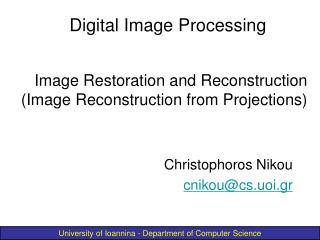
Digital Image Processing. Image Restoration and Reconstruction (Image Reconstruction from Projections). Christophoros Nikou cnikou@cs.uoi.gr. Contents. In this lecture we will look at image reconstruction from projections The reconstruction problem Principles of Computed Tomography (CT)

E N D
Digital Image Processing Image Restoration and Reconstruction(Image Reconstruction from Projections) Christophoros Nikou cnikou@cs.uoi.gr
Contents In this lecture we will look at image reconstruction from projections • The reconstruction problem • Principles of Computed Tomography (CT) • The Radon transform • The Fourier-slice theorem • Reconstruction by filtered back-projections
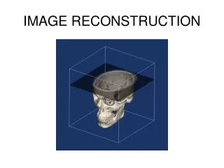
The Image Reconstruction Problem Consider a single object on a uniform background (suppose that this is a cross section of 3D region of a human body). Background represents soft, uniform tissue and the object is also uniform but with higher absorption characteristics.
The Image Reconstruction Problem (cont...) A beam of X-rays is emitted and part of it is absorbed by the object. The energy of absorption is detected by a set of detectors. The collected information is the absorption signal.
The Image Reconstruction Problem (cont...) A simple way to recover the object is to back-project the 1D signal across the direction the beam came. This simply means to duplicate the signal across the 1D beam.
The Image Reconstruction Problem (cont...) We have no means of determining the number of objects from a single projection. We now rotate the position of the source-detector pair and obtain another 1D signal. We repeat the procedure and add the signals from the previous back-projections. We can now tell that the object of interest is located at the central square.
The Image Reconstruction Problem (cont...) • By taking more projections: • the form of the object becomes clearer as brighter regions will dominate the result • back-projections with few interactions with the object will fade into the background.
The Image Reconstruction Problem (cont...) • The image is blurred. Important problem! • We only consider projections from 0 to 180 degrees as projections differing 180 degrees are mirror images of each other.
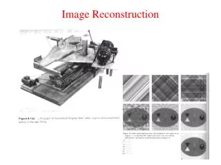
Principles of Computerized Tomography The goal of CT is to obtain a 3D representation of the internal structure of an object by X-raying it from many different directions. Imagine the traditional chest X-ray obtained by different directions. The image is the 2D equivalent of a line projections. Back-projecting the image would result in a 3D volume of the chest cavity.
Principles of Computerized Tomography (cont...) CT gets the same information by generating slices through the body. A 3D representation is then obtained by stacking the slices. More economical due to fewer detectors. Computational burden and dosage is reduced. Theory developed in 1917 by J. Radon. Application developed in 1964 by A. M. Cormack and G. N. Hounsfield independently. They shared the Nobel prize in Medicine in 1979.
The Radon Transform A straight line in Cartesian coordinates may be described by its slope-intercept form: or by its normal representation:
The Radon Transform (cont...) The projection of a parallel-ray beam may be modelled by a set of such lines. An arbitrary point (ρj,θk) in the projection signal is given by the ray-sum along the line xcosθk+ysinθk=ρj.
The Radon Transform (cont...) The ray-sum is a line integral:
The Radon Transform (cont...) For all values of ρand θwe obtain the Radon transform:
The Radon Transform (cont...) The representation of the Radon transform g(ρ,θ)as an image with ρand θas coordinates is called a sinogram. It is very difficult to interpret a sinogram.
The Radon Transform (cont...) Why is this representation called a sinogram? Image of a single point The Radon transform
The Radon Transform (cont...) The objective of CT is to obtain a 3D representation of a volume from its projections. The approach is to back-project each projection and sum all the back-projections to generate a slice. Stacking all the slices produces a 3D volume. We will now describe the back-projection operation mathematically.
The Radon Transform (cont...) For a fixed rotation angle θk, and a fixed distance ρj, back-projecting the value of the projection g(ρj,θk) is equivalent to copying the value g(ρj,θk) to the image pixels belonging to the line xcosθk+ysinθk=ρj.
The Radon Transform (cont...) Repeating the process for all values of ρj, having a fixed angle θk results in the following expression for the image values: This equation holds for every angle θ:
The Radon Transform (cont...) The final image is formed by integrating over all the back-projected images: Back-projection provides blurred images. We will reformulate the process to eliminate blurring.
The Fourier-Slice Theorem The Fourier-slice theorem or the central slice theorem relates the 1D Fourier transform of a projection with the 2D Fourier transform of the region of the image from which the projection was obtained. It is the basis of image reconstruction methods.
The Fourier-Slice Theorem (cont...) Let the 1D F.T. of a projection with respect to ρ(at a given angle) be: Substituting the projection g(ρ,θ) by the ray-sum:
The Fourier-Slice Theorem (cont...) Let now u=ωcosθandv=ωsinθ: which is the 2D F.T. of the image f(x,y) evaluated at the indicated frequencies u,v:
The Fourier-Slice Theorem (cont...) The resulting equation is known as the Fourier-slice theorem. It states that the 1D F.T. of a projection (at a given angle θ)is a slice of the 2D F.T. of the image.
The Fourier-Slice Theorem (cont...) We could obtain f(x,y) by evaluating the F.T. of every projection and inverting them. However, this procedure needs irregular interpolation which introduces inaccuracies.
Reconstruction byFiltered Back-Projections The 2D inverse Fourier transform of F(u,v) is Letting u=ωcosθandv=ωsinθ then the differential and
Reconstruction byFiltered Back-Projections (cont...) Using the Fourier-slice theorem: With some manipulation (left as an exercise, see the textbook): The term xcosθ+ysinθ=ρ and is independent of ω:
Reconstruction byFiltered Back-Projections (cont...) For a given angle θ, the inner expression is the 1-D Fourier transform of the projection multiplied by a ramp filter |ω|. This is equivalent in filtering the projection with a high-pass filter with Fourier Transform |ω| before back-projection.
Reconstruction byFiltered Back-Projections (cont...) Problem: the filter H(ω)=|ω| is not integrable in the inverse Fourier transform as it extends to infinity in both directions. It should be truncated in the frequency domain. The simplest approach is to multiply it by a box filter in the frequency domain. Ringing will be noticeable. Windows with smoother transitions are used.
Reconstruction byFiltered Back-Projections (cont...) An M-point discrete window function used frequently is When c=0.54, it is called the Hamming window. When c=0.5, it is called the Hann window. By these means ringing decreases.
Reconstruction byFiltered Back-Projections (cont...) Ramp filter multiplied by a box window Hamming window Ramp filter multiplied by a Hamming window
Reconstruction byFiltered Back-Projections (cont...) The complete back-projection is obtained as follows: Compute the 1-D Fourier transform of each projection. Multiply each Fourier transform by the filter function |ω| (multiplied by a suitable window, e.g. Hamming). Obtain the inverse 1-D Fourier transform of each resulting filtered transform. Back-project and integrate all the 1-D inverse transforms from step 3.
Reconstruction byFiltered Back-Projections (cont...) • Because of the filter function the reconstruction approach is called filtered back-projection (FBP). • Sampling issues must be taken into account to prevent aliasing. • The number of rays per angle which determines the number of samples for each projection. • The number of rotation angles which determines the number of reconstructed images.
Reconstruction byFiltered Back-Projections (cont...) Box windowed FBP Hamming windowed FBP Ringing is more pronounced in the Ramp FBP image
Reconstruction byFiltered Back-Projections (cont...) Box windowed FBP Hamming windowed FBP
Reconstruction byFiltered Back-Projections (cont...) Box windowed FBP
Reconstruction byFiltered Back-Projections (cont...) Hamming windowed FBP
Reconstruction byFiltered Back-Projections (cont...) Box windowed FBP Hamming windowed FBP There are no sharp transitions in the Shepp-Logan phantom and the two filters provide similar results.
Reconstruction byFiltered Back-Projections (cont...) Back-projection Ramp FBP Hamming FBP Notice the difference between the simple back-projection and the filtered back-projection.