Download
1 / 43
430 likes | 440 Views
SECCHI 3D Reconstruction Efforts at NRL. Angelos Vourlidas Naval Research Laboratory. With inputs from: R. Howard, J. Newmark, J. Cook, P. Reiser. Outline. Currently pursuing three approaches for 3D reconstructions of CMEs and coronal structures (plumes, streamers, etc).

E N D
SECCHI 3D Reconstruction Efforts at NRL Angelos Vourlidas Naval Research Laboratory With inputs from: R. Howard, J. Newmark, J. Cook, P. Reiser
Outline • Currently pursuing three approaches for 3D reconstructions of CMEs and coronal structures (plumes, streamers, etc). • Parametric modeling (RayTrace) Thernisien, Howard • Tomographic modeling (Pixon) Cook, Newmark, Reiser • Hybrid Approach (Pixon w/ ARM) Reiser
RayTrace • Models the brightness (total and polarized) produced by Thomson electron scattering from an arbitrary electron density distribution. • The input electron density distribution can be either a 3D data cube or an analytic description. • The output is a 2D image that simulates the observation in a white light coronagraph (user-defined). • The observer location, image spatial resolution, the orientation of the density model and the instrumental vignetting function are arbitrary. • Key contacts: Thernisien (raytrace), Patel (GUI), Howard, Vourlidas.
RayTrace Frontend From Thernisien et al. 2004
RayTrace Visualization • Example of a fluxrope visualization in RayTrace. From Thernisien et al. 2004
CME Models Currently Implemented • “2D” Loop • Spherical shell • Cylindrical shell • “Ice Cream Cone” • Graduated cylindrical shell (GCS) • Since the GCS model is a reasonable simulation of a flux-rope CME, we have used it to investigate the appearance of a CME as a function of STEREO separation angle. • Parameters are • The angular size in the two directions • Thickness of the shell • The height of the leading edge • The orientation of the structure in the corona • The radial electron density distribution
Spherical Shell O 10 2O 3O 6O 9O
“Flux Rope” Calculated in 3 Orientations O 1O 2O 9O 4O 7O
“Horizontal” Flux Rope • We present views of the horizontal flux rope as a function of angle from the observer’s viewpoint • A halo CME is 0 degrees • A limb CME is 90 degrees • The SECCHI COR2 vignetting function as been applied
Horizontal “Flux Rope” O 1O 2O 9O 4O 7O
RayTrace Summary • We have simulated the effect of the STEREO orbit separation on the appearance and the ability to reconstruct the 3D geometry • Spherical Shell, Loop, Cone and Graduated Cylinder give recognizable differences • Stereo separation angles of <20 degrees show little to no stereo effect. • Polarized Brightness (pB) images have little effect on CMEs at the limb, but considerable effect at large angles from the plane of the sky. • Complementary to 3D inversion and MHD techniques. • Could provide constraints to the MHD models.
Tomographic Modeling • Strategy: • Apply 3D tomographic electron density reconstruction techniques to solar features (mainly CMEs). • Utilize B, pB, temporal evolution from 2/3 vantage points. • Construct (time dependent) 3D electron density distribution. • Focus: • Use theoretical CME models and existing LASCO observations to identify the range of conditions and features where reconstruction techniques will be applicable. • Goal: • Provide a practical tool that will achieve ~daily CME 3D electron density models during the STEREO mission. • Key contacts: • J. Newmark, J. Cook, P. Reiser
Key Aspects • Renderer: • Physics (Thomson scattering), tangential and radial pB, total B, finite viewer geometry, optically thin plasma. • Reconstruction Algorithm: • PIXON (Pixon LLC), Pina, Puetter, Yahil (1993, 1995) - non-parametric, locally adaptive, iterative image reconstruction. • Chosen for speed (<10^9 voxels): small number of iterations, intelligent guidance to declining complexity per iteration. Sample times: 323 <15 min, 643 ~1 hr, 1283 ~6 hrs (1 GHz PC). • Minimum complexity: With this underdetermined problem, we make minimal assumptions in order to progress. Another possibility is forward modeling • Visualization: • 3D electron density distribution, time dependent (movies), multiple instrument, multiple spacecraft, physics MHD models.
3D Reconstruction: CME model (J. Chen)Three Orthogonal Viewpoints
3D Reconstruction: CME model (J. Chen)Three Ecliptic Viewpoints
Limitations • Limited viewpoints, underdetermined solution. Introduction of third vantage point helps with some objects. • Limited overlap region of multiple viewpoints. Objects outside one field of view. Intensity contributions from seen by only one telescope. S/C B S/C A Earth
Hybrid (ARM) Modeling • Recently we started exploring a 3rd approach to electron density reconstruction. • Namely, to incorporate a priori knowledge to the tomograhic method (Additional Regularization Method (ARM) ). • For example, we “know” • that electrons should be distributed smoothly along LOS, • that the emission should be positive, • that the large scale envelope of the CME should be symmetric. • Paul Reiser tested the effect of several constraints on synthetic data
A Priori Knowledge Let’s add two constraints: 1. Electron Density Distribution is Smooth 2. Axial Symmetry • But • Problem is underdetermined (2N2 equations, N3 unknowns) • Solutions are noisy
Another Example - Unmatched Scenes What to do when one viewpoint contains additional structure?
Conclusions • Useful 3D reconstructions are achievable! • Parametric modeling is easy to implement, fast, and intuitive. It can be directly linked to MHD models. Unlikely to match observations in detail. • Tomographic techniques achieve better agreement with observations. Time-consuming, error analysis is difficult/complex. • Incorporation of a priori knowledge in tomographic reconstruction shows great promise. Minimization subject to “magic” selection of parameters (different for each reconstruction). Still time-consuming • Tomographic reconstructions are significantly improved with the addition of a third viewpoint (LASCO continuing operation is extremely important). • Application to SECCHI will require substantial effort and collaboration; we appreciate all help on scientific preparations. • Web Site: http://stereo.nrl.navy.mil/ (follow link to 3D R&V). This contains past presentations and all necessary details to test reconstruction methods on our sample problems.
Backup Backup Slides
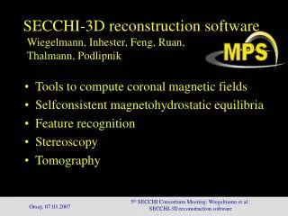
SECCHI Telescopes • The SECCHI suite consists of 5 telescopes to observe CMEs from their birth at the solar surface through the corona and into the inner heliosphere
Science - Examples • Geometric figures - uniform density, no background • Polar Plumes - hydrostatic equilibrium solution of density vs. height, tube expansion, statistics. • Equatorial streamers - projection of current sheets, effect of AR’s, compare to 3D reconstruction using tie points (Liewer 2001), density enhancements vs. folds. • CME’s – Use models to prepare for SECCHI, effect of viewpoint angles, velocity, polarization, structure evolution, etc. CME models include time dependence • J. Chen – CME, no background • P. Liewer – CME + background – not yet studied • Z. Mikic – CME, K corona evolution • S.T. Wu – CME - not yet studied • Questions: How to isolate CME? Assume subtraction of F+minimum K corona, but how to handle time dependent K corona? Why we want to: decrease complexity, eliminate structures of equal or greater brightness
3-D Reconstruction Using the Pixon Method • The problem is to invert the integral equation with noise: • But there are many more model voxels than data pixels. • And the reconstruction significantly amplifies the noise. • All reconstruction methods try to overcome these problems by restricting the model; they differ in how they do that. • A good first restriction is non-negative n(r). Non-Negative Least-Squares (NNLS) fit. • Minimum complexity (Ockham’s razor): restrict n(r) by minimizing the number of parameters used to define it. • The number of possible parameter combinations is large. An exhaustive parameter search is not possible. • The Pixon method is an efficient iterative procedure that approximates minimum complexity by finding the smoothest solution that fits the data (details: Puetter and Yahil 1999). • New modification: Adaptive (Hierarchical) Gridding
“Flux Rope” Calculated in Total B and pB O 1O 2O B pB 9O 4O 7O