Download
1 / 32
330 likes | 492 Views
Jeff Boody. 3D Reconstruction. Goals. Reconstruct 3D models from a sequence of at least two images No prior knowledge of the camera or scene Use the resulting 3D depth map as an input into the Biomimetic vision system. Overview. (1)Feature Extraction/ Matching. (2)Relating Images.

E N D
Jeff Boody 3D Reconstruction
Goals • Reconstruct 3D models from a sequence of at least two images • No prior knowledge of the camera or scene • Use the resulting 3D depth map as an input into the Biomimetic vision system
Overview (1)Feature Extraction/ Matching (2)Relating Images (3)Projective Reconstruction (6)3D Model Building (5)Dense Matching (4)Self-Calibration
Feature Extraction • Harris corner detector • Create gradient images Ix, Iy using convolution mask [-2, -1, 0, 1, 2] • Compute Ixx, Ixy, Iyy (smoothing optional) • The corner function: R(x,y) = det(x,y) - k trace(x,y)^2 • det(x,y) = Ixx(x,y) Iyy(x, y) – Ixy(x,y) Ixy(x,y) • trace(x,y) = Ixx(x,y) + Iyy(x,y) • Select local maxima over a threshold (vxl – adaptive) • Compute the sub-pixel location of corners
Feature Matching • Correlation • Compare features in I to features in I' that are within a search widow (approx 1/8th the image) • C = ∑∑ (I(x-i,y-j)-Imean)(I'(x-i,y-j)-I'mean) • The correlation score is summed over a region i=(-N,N), j=(-N,N), where N = 3 • Zhang's robust matching • Correlation, strength/unambiguity of matches, iterative relaxation • Eliminates ambiguity caused by multiple matches
Relating Images(1) • Fundamental matrix • u'TFu = 0 • uu'F11 + uv'F21 + uF31 + vu'F12 + vv'F22 + vF32 + u'F13 + v'F23 + F33 = 0 • Af = 0, (uu', uv', u, vu', vv', v, u', v', 1) • ||f|| = 1, (F is only defined up to an unknown scale) • det(F) = 0 (singularity constraint, rank 2) • The epipoles are the left and right null spaces of F
Relating Images(2) • 8-Point Algorithm • Normalize points, u = T1 u, u' = T2 u' • Points are translated to their centroid • Points are scaled so their average distance from the origin is √2 • Solve Af = 0, using SVD (A = UDVT, F is V9) • Take the SVD of F (F = UDVT) and set the smallest eigenvalue to 0, corresponding to the closest singular matrix under the Frobenius norm (||F|| = 1) • De-normalize F, F = T2T F T1
Relating Images(3) • 7-Point Algorithm • Same as the 8-point algorithm, except det(F) = 0 is enforced differently, and only 7 point correspondences are required • F = aF1 + (1-a)F2, where F1 and F2 are V9 and V8 respectively • Enforce the singularity constraint by solving det(aF1 + (1-a)F2) = 0 for a • This leads to a cubic equation in a that has one or three real solutions
Relating Images(4) • In practice we have many more matches then 8, some of which can be noisy (є). • Ransac or Least Median Squares (to name a few) • N is the number of matches • m is the number of samples chosen • p is the sample size (i.e. 7 or 8) • є is the percentage of outliers
Relating Images(5) • Ransac • while(1 - (1 - (1 - є)^p)^m < 0.95) • Select random sample (bucketing) • Solve for FM • Determine inliers (over all matches) • Matches that are within a given threshold (typically 1 or 2 pixels) are chosen as inliers • Keep the FM which has the largest number of inliers
Relating Images(6) • Least Median Squares • The same loop as Ransac can be used • Inliers are chosen as follows • Calculate the residuals for every match, and compute the median • б = 1.4826(1 + 5 / (N-p))√MJ • inlier if ri2 ≤ (2.5б)2, outlier otherwise • Select the FM for which the inliers minimize ∑ri2
Relating Images(7) • Distance metric: Euclidean distance from the point u' to its epipolar line Fu • Fu ~ l', FTu' ~ l • d(u', Fu) = |u'TFu| / √((Fu)21 + (Fu)22) • Residual • ri2 = d2(u'i, Fui) + d2(ui, FTu'i)
Relating Images(8) • Non-linear minimization (Levenberg-Marquardt) • Often, the fundamental matrix that was found using the robust method is still not good enough • Noise in the input data, outliers might not be detected, errors in setting the singularity constraint, ... • Parameterize F = • Solve min d2(u'i, Fui) + d2(ui, FTu'i), for inlier matches • The solution requires taking the derivative of the distance metric and possibly using up to 36 different parameterizations of F (i.e. epipoles at infiniti)
Projective Reconstruction(1) • Projective Transform • x = PX • P1M = K[I3 | 03] • P2M = K[RT | -RT t] • K =
Projective Reconstruction(2) • Initial projection matrices (first method) • Normalize images: m = K*-1m • P1 = [I3 | 03] • P2 = [[e2]xF + e2 piT | sigma e2] • Choose pi such that: [e2]xF + e2 piT = R* = I • sigma can be arbitrarily set to 1, cx = Image.width/2, cy = Image.height/2, s = 0, aspect ratio = 1 • For the focal length, several guesses must be tried, keeping the one with the most points reconstructed
Projective Reconstruction(3) • Initial structure (first method) • u = PX where u = w(u,v,1)T, X = (x, y, z, w)T • wu = p1TX, wv = p2TX, w = p3TX • Each point in each view results in • [up3T-p1T]X = 0, [vp3T-p2T]X = 0 • Resulting in this set of linear equations: AX = 0 • M is number of points, N is number of views • A is 2N x 4M, X is 4M x 1
Projective Reconstruction(4) • Perspective Factorization (second method)
Projective Reconstruction(5) • Perspective Factorization (second method)
Projective Reconstruction(6) • Other algorithms in projective reconstruction • Triangulation: a more robust method for reconstructing the initial structure • Iterated Extended Kalman Filters: a method to update the structure when more than two views are available • Bundle Adjustment: another non-linear minimization of the structure which requires the solution to take advantage of the sparse structure of the problem matrix. Otherwise, for a typical image sequence, the solution must be minimized over more than 6000 variables
Self-calibration(1) • Self-calibration is the process that upgrades a projective reconstruction to a metric reconstruction
Self-calibration(2) • The image of the absolute conic
Self-calibration(3) • Constraints on the DIAC • n x (#known) + (n - 1) x (#fixed) >= 8
Self-calibration(4) • Linear algorithm
Self-calibration(5) • Linear algorithm
Self-calibration(6) • Example critical motion sequences • Pure translation: Scaling of optical axis (1 DOF) • Pure rotation: Arbitrary position of PI (3 DOF) • Orbital motion: ? • Planar motion: ?
Results(1) • Feature extraction (first and third images)
Results(2) • Feature matching
Results(3) • Inliers after Ransac
Results(4) • Inliers after tracking
Results(5) • Epipolar lines
Results(6) • Metric reconstruction using 3 virtual cameras
Future Work • Finish projective reconstruction and self-calibration algorithms • Non-linear minimization for FM, projective reconstruction, self-calibration • Dense matching (image rectification followed by correlation along epipolar lines) • Model building (Delunay triangulation) • Critical motion sequences