Download

1 / 22
280 likes | 579 Views
Artificial Neural Networks. Introduction Design of Primitive Units Perceptrons The Backpropagation Algorithm Advanced Topics. Basics. In contrast to perceptrons, multilayer networks can learn not only multiple decision boundaries, but the boundaries may be nonlinear. Output nodes.

E N D
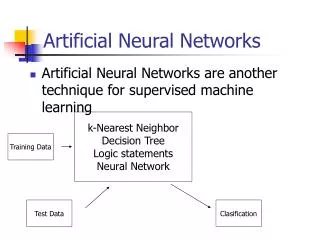
Artificial Neural Networks • Introduction • Design of Primitive Units • Perceptrons • The Backpropagation Algorithm • Advanced Topics
Basics In contrast to perceptrons, multilayer networks can learn not only multiple decision boundaries, but the boundaries may be nonlinear. Output nodes Internal nodes Input nodes
Example x2 x1
One Single Unit To make nonlinear partitions on the space we need to define each unit as a nonlinear function (unlike the perceptron). One solution is to use the sigmoid unit. x1 w1 x2 net w2 Σ O = σ(net) = 1 / 1 + e -net w0 wn xn X0=1
More Precisely O(x1,x2,…,xn) = σ ( WX ) where: σ ( WX ) = 1 / 1 + e -WX Function σ is called the sigmoid or logistic function. It has the following property: d σ(y) / dy = σ(y) (1 – σ(y))
Backpropagation Algorithm Goal: To learn the weights for all links in an interconnected multilayer network. We begin by defining our measure of error: E(W) = ½ Σd Σk (tkd – okd) 2 k varies along the output nodes and d over the training examples. The idea is to use again a gradient descent over the space of weights to find a global minimum (no guarantee).
Output Nodes Output nodes
Algorithm The idea is to use again a gradient descent over the space of weights to find a global minimum (no guarantee). • Create a network with nin input nodes, nhidden internal nodes, • and nout output nodes. • Initialize all weights to small random numbers. • Until error is small do: • For each example X do • Propagate example X forward through the network • Propagate errors backward through the network
Propagating Forward Given example X, compute the output of every node until we reach the output nodes: Output nodes Compute sigmoid function Internal nodes Input nodes Example X
Propagating Error Backward • For each output node k compute the error: • δk = Ok (1-Ok)(tk – Ok) • For each hidden unit h, calculate the error: • δh = Oh (1-Oh) Σk Wkh δk • Update each network weight: • Wji = Wji + ΔWji • where ΔWji = η δj Xji (Wji and Xji are the input and • weight of node i to node j)
Adding Momentum • The weight update rule can be modified so as to depend • on the last iteration. At iteration n we have the following: • ΔWji (n) = η δj Xji + αΔWji (n) • Where α ( 0 <= α <= 1) is a constant called the momentum. • It increases the speed along a local minimum. • It increases the speed along flat regions.
Remarks on Backpropagation • It implements a gradient descent search over the weight space. • It may become trapped in local minima. • In practice, it is very effective. • 4. How to avoid local minima? • Add momentum • Use stochastic gradient descent • Use different networks with different initial values • for the weights.
Representational Power • Boolean functions. Every boolean function can be represented • with a network having two layers of units. • Continuous functions. All bounded continuous functions can also • be approximated with a network having two layers of units. • Arbitrary functions. Any arbitrary function can be approximated • with a network with three layers of units.
Hypothesis Space • The hypothesis space is a continuous space, as opposed to the discrete space explored by decision trees and the candidate elimination algorithm. • The bias is a smooth “similarity based bias” meaning points close to each other are expected to share the same class.
Example Again x2 x1 Smooth regions
Hidden Representations An interesting property of neural networks is their ability to capture intermediate representations within the hidden nodes. 10000000 01000000 00100000 00010000 00001000 00000100 00000010 00000001 10000000 01000000 00100000 00010000 00001000 00000100 00000010 00000001 Hidden nodes The hidden nodes encode each number using three bits.
Node Evolution Different units Error iterations Different weights weight iterations
Generalization and Overfitting One obvious stopping point for backpropagation is to continue iterating until the error is below some threshold; this can lead to overfitting. Validation set error Error Training set error Number of weight updates
Solutions • Use a validation set and stop until the error is small in this set. • Use 10 fold cross validation • Use weight decay; the weights are decreased slowly on each iteration.
Artificial Neural Networks • Introduction • Design of Primitive Units • Perceptrons • The Backpropagation Algorithm • Advanced Topics
Advanced Topics • Alternative error functions, correcting the derivative of the function, minimizing cross entropy, etc. • Dynamically modify the network structure. • Recurrent Networks • Apply to time series analysis • The output at time t serves as input to other units at time t+1
Recurrent Network y(t+1) x(t)