Download
1 / 37

E N D
Commercial ANNs • Commercial ANNs incorporate three and sometimes four layers, including one or two hidden layers. Each layer can contain from 10 to 1000 neurons. Experimental neural networks may have five or even six layers, including three or four hidden layers, and utilise millions of neurons.
Example • Character recognition
Problems that are not linearly separable • Xor function is not linearly separable • Using Multilayer networks with back propagation training algorithm • There are hundreds of training algorithms for multilayer neural networks
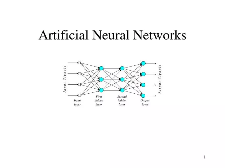
Multilayer neural networks • A multilayer perceptron is a feedforward neural network with one or more hidden layers. • The network consists of an input layer of source neurons, at least one middle or hidden layer of computational neurons, and an output layer of computational neurons. • The input signals are propagated in a forward direction on a layer-by-layer basis.
What do the middle layers hide? A hidden layer “hides” its desired output. Neurons in the hidden layer cannot be observed through the input/output behaviour of the network. There is no obvious way to know what the desired output of the hidden layer should be.
Back-propagation neural network • Learning in a multilayer network proceeds the same way as for a perceptron. • A training set of input patterns is presented to the network. • The network computes its output pattern, and if there is an error or in other words a difference between actual and desired output patterns the weights are adjusted to reduce this error.
In a back-propagation neural network, the learning algorithm has two phases. • First, a training input pattern is presented to the network input layer. The network propagates the input pattern from layer to layer until the output pattern is generated by the output layer. • If this pattern is different from the desired output, an error is calculated and then propagated backwards through the network from the output layer to the input layer. The weights are modified as the error is propagated.
The back-propagation training algorithm Step 1: Initialisation Set all the weights and threshold levels of the network to random numbers uniformly distributed inside a small range: where Fi is the total number of inputs of neuron i in the network. The weight initialisation is done on a neuron-by-neuron basis.
Three-layer network w13 = 0.5, w14 = 0.9, w23 = 0.4, w24 = 1.0, w35 = 1.2, w45 = 1.1, 3 = 0.8, 4 = 0.1 and 5 = 0.3
The effect of the threshold applied to a neuron in the hidden or output layer is represented by its weight, , connected to a fixed input equal to 1. • The initial weights and threshold levels are set randomly e.g., as follows: • w13 = 0.5, w14 = 0.9, w23 = 0.4, w24 = 1.0, w35 = 1.2, w45 = 1.1, 3 = 0.8, 4 = 0.1 and 5 = 0.3.
Step 2: Activation Activate the back-propagation neural network by applying inputs x1(p), x2(p),…, xn(p) and desired outputs yd,1(p), yd,2(p),…, yd,n(p). (a) Calculate the actual outputs of the neurons in the hidden layer: where n is the number of inputs of neuron j in the hidden layer, and sigmoid is the sigmoid activation function.
Step 2: Activation (continued) (b) Calculate the actual outputs of the neurons in the output layer: where m is the number of inputs of neuron k in the output layer.
If the sigmoid activation function is used the output of the hidden layer is And the actual output of neuron 5 in the output layer is And the error is
What learning law applies in a multilayer neural network?
Step 3: Weight training output layer Update the weights in the back-propagation network propagating backward the errors associated with output neurons. (a) Calculate the error and then the error gradient for the neurons in the output layer: Then the weight corrections: Then the new weights at the output neurons:
The error gradient for neuron 5 in the output layer: • Determine the weight corrections assuming that the learning rate parameter, , is equal to 0.1:
Apportioning error inthe hidden layer • Error is apportioned in proportion to the weights of the connecting arcs. • Higher weight indicates higher error responsibility
Step 3: Weight training hidden layer (b) Calculate the error gradient for the neurons in the hidden layer: Calculate the weight corrections: Update the weights at the hidden neurons:
The error gradients for neurons 3 and 4 in the hidden layer: • Determine the weight corrections:
= + D = + = w w w 0 . 5 0 . 0038 0 . 5038 13 13 13 = + D = - = w w w 0 . 9 0 . 0015 0 . 8985 14 14 14 = + D = + = w w w 0 . 4 0 . 0038 0 . 4038 23 23 23 = + D = - = w w w 1 . 0 0 . 0015 0 . 9985 24 24 24 = + D = - - = - w w w 1 . 2 0 . 0067 1 . 2067 35 35 35 = + D = - = w w w 1 . 1 0 . 0112 1 . 0888 45 45 45 q = q + D q = - = 0 . 8 0 . 0038 0 . 7962 3 3 3 q = q + D q = - + = - 0 . 1 0 . 0015 0 . 0985 4 4 4 q = q + D q = + = 0 . 3 0 . 0127 0 . 3127 5 5 5 • At last, we update all weights and threshold: • The training process is repeated until the sum of squared errors is less than 0.001.
Step 4: Iteration Increase iteration p by one, go back to Step 2 and repeat the process until the selected error criterion is satisfied. As an example, we may consider the three-layer back-propagation network. Suppose that the network is required to perform logical operation Exclusive-OR. Recall that a single-layer perceptron could not do this operation. Now we will apply the three-layer net.
Network represented by McCulloch-Pitts model for solving the Exclusive-OR operation
Accelerated learning in multilayer neural networks • A multilayer network learns much faster when the sigmoidal activation function is represented by a hyperbolic tangent: • where a and b are constants. • Suitable values for a and b are: • a = 1.716 and b = 0.667
We also can accelerate training by including a momentum term in the delta rule: where is a positive number (0 1) called the momentum constant. Typically, the momentum constant is set to 0.95. This equation is called the generalised delta rule.
Learning with an adaptive learning rate To accelerate the convergence and yet avoid the danger of instability, we can apply two heuristics: Heuristic If the error is decreasing the learning rate , should be increased. If the error is increasing or remaining constant the learning rate , should be decreased.
Adapting the learning rate requires some changes in the back-propagation algorithm. • If the sum of squared errors at the current epoch exceeds the previous value by more than a predefined ratio (typically 1.04), the learning rate parameter is decreased (typically by multiplying by 0.7) and new weights and thresholds are calculated. • If the error is less than the previous one, the learning rate is increased (typically by multiplying by 1.05).
Typical Learning with adaptive learning rate plus momentum