Download
1 / 31
360 likes | 511 Views
Artificial Neural Networks. Dr. Lahouari Ghouti Information & Computer Science Department. Review of Probability Concepts. Why Probabilities. The world is a very uncertain place 30 years of Artificial Intelligence, Machine Learning and Data-mining research evolved around this fact!

E N D
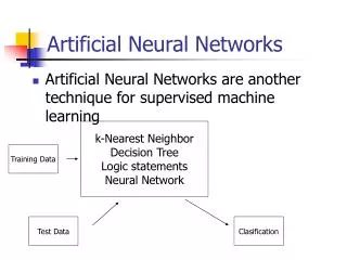
Artificial Neural Networks Dr. Lahouari Ghouti Information & Computer Science Department Review of Basic Concepts
Review of Probability Concepts Review of Basic Concepts
Why Probabilities • The world is a very uncertain place • 30 years of Artificial Intelligence, Machine Learning and Data-mining research evolved around this fact! • • And then few “daring” researchers decided to • use some ideas from the eighteenth century! Review of Basic Concepts
Why Probabilities (Cont’d) • We will review the fundamentals of probability. • • It’s really going to be worth it! • • In this lecture, you’ll see an example of probabilistic analytics in action: Conditional Probabilities in Real Life? Review of Basic Concepts
Discrete Random Variables • A is a Boolean-valued random variable if A denotes an event, and there is some degree of uncertainty as to whether A occurs. • Examples: • A = You will all get A+ in this course • A = You wake up tomorrow with a headache • A = You have a strong fever Review of Basic Concepts
Probabilities • We write P(A) as “the fraction of possible worlds in which A is true” • We could at this point spend 2 hours on the philosophy of this. Event Space of all possible worlds P(A) = Colored Area Area = 1 Review of Basic Concepts
The Axioms of Probability • 0 <= P(A) <= 1 • P(True) = 1 • P(False) = 0 • P(A or B) = P(A) + P(B) - P(A and B) Review of Basic Concepts
Interpreting the Axioms • 0 <= P(A) <= 1 • P(True) = 1 • P(False) = 0 • P(A or B) = P(A) + P(B) - P(A and B) The area of A can’t get any smaller than 0 Note: A zero area would mean no world could ever have A true! Review of Basic Concepts
Interpreting the Axioms (Cont’d) • 0 <= P(A) <= 1 • P(True) = 1 • P(False) = 0 • P(A or B) = P(A) + P(B) - P(A and B) The area of A can’t get any bigger than 1 Note: An area of 1 would mean all worlds will have A true! Review of Basic Concepts
Interpreting the Axioms (Cont’d) • 0 <= P(A) <= 1 • P(True) = 1 • P(False) = 0 • P(A or B) = P(A) + P(B) - P(A and B) Review of Basic Concepts
Other Methodologies • There have been attempts to do different methodologies for uncertainty: • Fuzzy Logic • Three-valued logic • Dempster-Shafer • Non-monotonic reasoning Review of Basic Concepts
Theorems from the Axioms • 0 <= P(A) <= 1, P(True) = 1, P(False) = 0 • P(A or B) = P(A) + P(B) - P(A and B) • P(not A) = P(~A) = 1-P(A) Review of Basic Concepts
Multivalued Random Variables • Suppose A can take on more than 2 values • A is a random variable with arity k if it can take on exactly one value out of {v1, v2, …, vk } • P(A= vi and A= vj) = 0 if i j • P(A= v1 or A= v2 or … or A= vk) = 1 Review of Basic Concepts
Conditional Probabilities • P(A|B) = Fraction of worlds in which B is true that also have A true • Example: H = “Have a headache” F = “Coming down with Flu” Review of Basic Concepts
Conditional Probabilities (Cont’d) • P(A|B) = Fraction of worlds in which B is true that also have A true: Corollary: The Chain Rule Review of Basic Concepts
Conditional Probabilities (Cont’d) • Calculations Area-Wise: • P(F) = “Coming down with Flu” = A+B • P(H) = “Having a Headache” = B + C • Then, we have: • Now, how can we get: Review of Basic Concepts
Bayes Rule Bayes, Thomas (1763): An essay towards solving a problem in the doctrine of chances. Philosophical Transactions of the Royal Society of London, 53:370-418 Review of Basic Concepts
Log Probabilities Since probabilities of datasets get so small we usually use log probabilities Review of Basic Concepts
Independently Distributed Data Let x[i] denote the i’th field of record x. For indepently-distributed data, x[i] is independent of {x[1],x[2],..x[i-1], x[i+1],…x[M]} Assume A and B are Boolean Random Variables. Then “A and B are independent” if and only if: Review of Basic Concepts
Expectations and Covariance • The expectation of a function f(x) is the average value of f(x) under a probability distribution p(x). It is given by weighted by the relative probabilities of the different values of x. Review of Basic Concepts
Expectations and Covariance (Cont’d) • Ex [f(x,y)] the average of the function f(x,y) with respect to the distribution of x. Ex [f(x,y)] is a function of y. • var[f] = E[(f(x) – E[f(x)]2(] the variance of f(x) = E[f(x)2] - E[f(x)]2 var[x] = E[x2] - E[x]2 Review of Basic Concepts
Expectations and Covariance (Cont’d) • The covariance of two random variables x and y cov[x,y] = Ex,y [{x – E[x]} {y – E[y]}] = Ex,y [xy] – E[x] E[y] expresses the extent to which x and y vary together. If x and y are independent then their covariance vanishes. When x and y are vectors (Vector Notation): cov[x,y] = Ex,y [{x – E[x]} {yT – E[yT]}] = Ex,y [xyT] – E[x] E[yT] Review of Basic Concepts
Signal & Weight Vector Spaces Vectors in n.
Vector Space • An operation called vector addition is defined such that if • x X and y X then x+y X. • x + y = y + x • (x + y) + z = x + (y + z) • There is a unique vector 0 X, called the zero vector, such • that x + 0 = x for all x X. • For each vector there is a unique vector in X, to be called • (-x ), such that x + (-x ) = 0 .
Vector Space (Cont’d) • An operation, called multiplication, is defined such that • for all scalars a F, and all vectors x X, a x X. • For any x X , 1x = x (for scalar 1). • For any two scalars a F and b F, and any x X, • a (bx) = (a b) x . • (a + b) x = a x + b x . • a (x + y) = a x + a y
Other Vector Spaces • Polynomials of degree 2 or less. • Continuous functions in the interval [0,1]. • Name other spaces….
Linear Independence • If the following relation: implies that each Then: Is a set of linearly independent vectors.
Linear Independence (Cont’d) • Let’s consider the following example: Let: This can only be true if
Basis Vectors • A set of basis vectors for the space X is a set of vectors which spans • X and is linearly independent. • The dimension of a vector space, Dim(X), is equal to the number of • vectors in the basis set. • Let X be a finite dimensional vector space, then every basis set of • X has the same number of elements. • An Example: • Polynomials of degree 2 or less. • Basis:
Inner Product / Norm • A scalar function of vectors x and y can be defined as an inner product, (x,y), provided the following are satisfied (for real inner products): • (x, y) = (y, x). • (x, ay1+by2) = a(x ,y1) + b(x ,y2) . • (x , x) ≥ 0 , where equality holds iff x = 0 . • A scalar function of a vector x is called a norm, ||x||, provided the following are satisfied: ||x|| ≥ 0 ||x|| = 0 iff x = 0 ||a x|| = |a| ||x|| for scalar a ||x + y|| ||x|| ||y||
Orthogonality Two vectors x, y X are orthogonal if (x,y) = 0 .