Download
1 / 24
260 likes | 542 Views
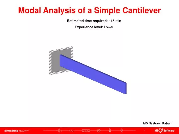
Modal Analysis of a Simple Cantilever. Estimated time required : ~15 min Experience level: Lower. MD Nastran / Patran. Topics Covered. Creating surface with XYZ method Performing a Modal Analysis Displaying Modal Analysis results Obtaining results from *.f06 file. Problem Description. y.

E N D
Modal Analysis of a Simple Cantilever Estimated time required: ~15 min Experience level: Lower MD Nastran / Patran
Topics Covered • Creating surface with XYZ method • Performing a Modal Analysis • Displaying Modal Analysis results • Obtaining results from *.f06 file
Problem Description y h=0.1m x L = 1.0 m • The beam below is cantilevered or "built in" on the left edge. • Material properties for aluminum: • Modulus of Elasticity = 70 x 109 Pa • Density = 2700 kg/m3 • Poisson Ratio = 0.3 • The beam has a solid rectangular cross section with thickness (z-direction) t = 0.01 meters and height (y-direction) h = 0.1 meters.
Expected Results First Mode Frequency = 8.19 Second Mode Frequency = 49.912
Creating a New Database a • Click File menu / Select New. • In the File name text field enter modal_beam • Click OK. b c
Database Settings for the Model • Select Tolerance radio button: Based on Model • Enter in the Approximate MaximumModel Dimension text field: 1 • Select Analysis Code to be MSC.Nastran from the drop down menu • Select Analysis Type to be Thermal from the drop down menu. • Click OK. a b c d e Remember: MSC.Patran does not handle units of measurement, so it is essential to remember to use one consistent system of measurement. In this example, SI units are used with the following measuring units: Remember: MSC.Patran does not handle units of measurement, so it is essential to remember to use one consistent system of measurement. In this example, SI units are used with the following measuring units: Input Output Length meters Force Newtons Elastic Modulus Pa Mass kg Displacement meters Force Newtons Stress Pa
Creating Surface a • Click on Geometry icon • Select Create / Surface / XYZ from the drop down menus • In the Vector Coordinate List text field enter <1 0.1 0> • Click on Auto Execute checkbox to turn Off • In the Origin Coordinate List text field enter [0 0 0] • Click on Apply b c d e f
Creating Mesh Seed a • Click on Elements icon • Select Create / Mesh Seed / Uniform from the drop down menus • Click on Number of Elements radio button • In the Number text field enter 6 • Click on Auto Execute checkbox to turn it off • In the Curve List text field select the bottom curve (surface1.4) • Click Apply b c d e f g
Creating Mesh Seed a • Select Create / Mesh Seed / Uniform from the drop down menus • Click on Number of Elements radio button • In the Number text field enter 1 • In the Curve List text field select the left curve (surface1.1) • Click Apply b c e
Creating Mesh • Select Create / Mesh / Surface from the drop down menu • In Element Shape select Quad • In Mesher select IsoMesh • In Topology select Quad4 • In the Surface List text field select the entire surface (surface 1) • Click Apply a b c d e f Note: The Global Edge Length can be ignored since the planted mesh seeds have priority over the mesh density
Equivalence the Surface Mesh • Select Equivalence / All / ToleranceCube from the drop down menus • In the Equivalence Tolerance text field enter 0.003 • Click Apply • In the Command History window make sure that 0 nodes were deleted a b c Note: No nodes have been deleted because a single surface has been meshed and no coincident nodes exist. d
Applying Cantilevered Boundary Condition a • Click on Loads/BCs icon • Select Create / Displacement / Nodal from the drop down menus • In the New Set Name text field enter cantilever • Click on Input Data button • In the Translations text field enter <0 0 0> • In the Rotations text field enter <0 0 0> • Click Ok button • Click Select Application Region button • Under Geometry Filter, click on FEM radio button • In Select Nodes text field select the two left nodes of the surface • Click Add button • Click Ok button • Click Apply button b i e f j k g l c d h m
Boundary Condition Summary • The two nodes at the left side are constrained in 1 2 3 4 5 6 which are the respective XYZ for translation and rotation a
Creating Aluminum Material Properties a • Click on Materials icon • Select Create / Isotropic / Manual Input from the drop down menu • In the Material Name text field enter aluminum • Click on Input Properties button • In Elastic Modulus text field enter 70e9 • In Poisson Ratio text field enter 0.3 • In Density text field enter 2700 • Click Ok button • Click Apply button b e f g c h d i
Applying Properties a • Click on Properties Icon • Select Create / 2D / Shell from the drop down menu • In Property Set Name text field enter plate_prop • Click on Input Properties button • Click on Select Material icon • Click on aluminum • In the Thickness text field enter 0.01 • Click Ok button • In Select Members text field select the surface (surface 1) • Click Add button • Click Apply button e b g f c h d i j k
Analyzing Model a • Click Analysis icon • Select Analyze / Entire Model / Full Run from the drop down menus • Click on Solution Type button • Click on Normal Modes radio button • Click Ok button • Click Apply button b d e v f
Attaching Result Files a • Select Access Results / Attach XDB / Result Entitites from the drop down menu • Click on Select Results File button • Double-click on modal_beam.xdb • Click on Apply button c b d
Creating Fringe Plots of Modal Analysis – First Mode a • Click Results icon • Select Create / Quick Plot from the drop down menu • Under Select Result Cases click on Default, A1:Mode1: Freq = 8.19 • Under Fringe Results select Eigenvectors, Translational • Under Select Deformation Result click on Eigenvectors, Translational • Click Apply button b c d e Note: The results that you obtain might differ slightly from those shown here f
Creating Fringe Plots of Modal Analysis – Second Mode • Select Create / Quick Plot from the drop down menu • Under Select Result Cases click on Default, A1:Mode2: Freq = 49.912 • Under Fringe Results select Eigenvectors, Translational • Under Select Deformation Result click on Eigenvectors, Translational • Click Apply button Note: The results that you obtain might differ slightly from those shown here
Viewing Results in *f06 file To obtain detailed results information about the analysis, you can create a report file with the needed information or open the *f06 file to obtain the real eigenvalues. These are the natural frequencies (in radians) or the beam.
Summary of Results of FEA on Given Truss Model First Mode Frequency = 8.19 Second Mode Frequency = 49.912
Important Skills Acquired • Creating surface with XYZ method • Performing a Modal Analysis • Displaying Modal Analysis results • Obtaining results from *.f06 file
Further Analysis (Optional) • Study the first 5 modes shapes produced by MSC.Nastran and comment on which modes are not associated with bending about the minimum “I” direction. • Rerun the analysis using twice as many elements. Does a refinement in the mesh appear to produce more accurate results? • Change the Poisson’s ratio to 0.0. Rerun the analysis using the original global edge length (6 elements). Compare these errors with the errors found while using a Poisson’s ratio of 0.3. Propose explanation for the differences.
Best Practices • Keep a consistent system of units • Remember to choose the solution type adequately so that MD Nastran knows what type of solution type its solving for • Check your answer by doing hand calculations to determine if the answers obtained are within the spectrum of acceptance.