Download
1 / 86
1.1k likes | 1.49k Views
Experimental Modal Analysis. f(t). x(t). m. c. k. + +. +. +. =. SDOF and MDOF Models Different Modal Analysis Techniques Exciting a Structure Measuring Data Correctly Modal Analysis Post Processing. 1 T. 1 T n. Simplest Form of Vibrating System. Displacement.

E N D
f(t) x(t) m c k + + + + = SDOF and MDOF Models Different Modal Analysis Techniques Exciting a Structure Measuring Data Correctly Modal Analysis Post Processing
1 T 1 Tn Simplest Form of Vibrating System Displacement Displacement d = D sinnt D Time T Frequency m Period, Tn in [sec] k Frequency, fn= in [Hz = 1/sec] k n= 2 fn = m
Mass and Spring time m1 m Increasing mass reduces frequency
time m k c1 + c2 Mass, Spring and Damper Increasing damping reduces the amplitude
f(t) x(t) m c k Acceleration Vector Velocity Vector Displacement Vector Applied force Vector Basic SDOF Model M = mass (force/acc.) C = damping (force/vel.) K = stiffness (force/disp.)
f(t) x(t) m 1 k c k 1 2m 1 c |H()| H() 0 = k/m 0º – 90º – 180º SDOF Models — Time and Frequency Domain F() X() H()
X4 X3 X2 X1 H22 F3 H21 Modal Matrix Modal Model (Freq. Domain)
MDOF Model Magnitude 1+2 d1+ d2 1 2 Frequency m d1 Phase Frequency dF 0° -90° -180° 2 1 1+2
Rotor Bearing Bearing 2 1 q2 Foundation Why Bother with Modal Models? Modal Space = Simplicity Physical Coordinates = CHAOS 1 1 q1 3 1 q3
Definition of Frequency Response Function F(f) H(f) X(f) F X f f f H(f) is the system Frequency Response Function F(f) is the Fourier Transform of the Input f(t) X(f) is the Fourier Transform of the Output x(t)
Benefits of Frequency Response Function • Frequency Response Functions are properties of linear dynamic systems • They are independent of the Excitation Function • Excitation can be a Periodic, Random or Transient function of time • The test result obtained with one type of excitation can be used for predicting the response of the system to any other type of excitation F(f) H(f) X(f)
Different Forms of an FRF Compliance Dynamic stiffness (displacement / force) (force / displacement) MobilityImpedance (velocity / force) (force / velocity) Inertance or ReceptanceDynamic mass (acceleration / force) (force /acceleration)
Alternative Estimators H(f) F(f) X(f)
Alternative Estimators + H(f) F(f) X(f) N(f) SISO: MIMO:
Alternative Estimators + H(f) F(f) X(f) M(f) SISO: MIMO:
Which FRF Estimator Should You Use? Accuracy Definitions: Accuracy for systems with: H1 H2 H3 Input noise - Best - Output noise Best - - Input + output noise - - Best Peaks (leakage) - Best - Valleys (leakage) Best - - User can choose H1, H2 or H3 after measurement
f(t) x(t) m c k + + + + = SDOF and MDOF Models Different Modal Analysis Techniques Exciting a Structure Measuring Data Correctly Modal Analysis Post Processing
Three Types of Modal Analysis • Hammer Testing • Impact Hammer ’taps’...serial or parallel measurements • Excites wide frequency range quickly • Most commonly used technique • Shaker Testing • Modal Exciter ’shakes’ product...serial or parallel measurements • Many types of excitation techniques • Often used in more complex structures • Operational Modal Analysis • Uses natural excitation of structure...serial or parallel measurements • ’Cutting’ edge technique
Different Types of Modal Analysis (Pros) • Hammer Testing • Quick and easy • Typically Inexpensive • Can perform ‘poor man’ modal as well as ‘full’ modal • Shaker Testing • More repeatable than hammer testing • Many types of input available • Can be used for MIMO analysis • Operational Modal Analysis • No need for special boundary conditions • Measure in-situ • Use natural excitation • Can perform other tests while taking OMA data
Different Types of Modal Analysis (Cons) • Hammer Testing • Crest factors due impulsive measurement • Input force can be different from measurement to measurement (different operators, difficult location, etc.) • ‘Calibrated’ elbow required (double hits, etc.) • Tip performance often an overlooked issue • Shaker Testing • More difficult test setup (stingers, exciter, etc.) • Usually more equipment and channels needed • Skilled operator(s) needed • Operational Modal Analysis • Unscaled modal model • Excitation assumed to cover frequency range of interest • Long time histories sometimes required • Computationally intensive
Inverse FFT Time Domain Frequency Domain Frequency Response Function FFT Output Input FFT
Roving hammer method: Response measured at one point Excitation of the structure at a number of points by hammer with force transducer First Mode Second Mode Third Mode Force Force Force Force Force Modal Domain View Frequency Domain View Force Force Force Force Force Force Force Hammer Test on Free-free Beam • FRF’s between excitation points and measurement point calculated • Modes of structure identified Amplitude Distance Beam Frequency Acceleration Press anywhere to advance animation
Measurement of FRF Matrix (SISO) One row • One Roving Excitation • One Fixed Response (reference) SISO X1 H11 H12 H13 ...H1nF1 X2 H21 H22 H23 ...H2n F2 X3 H31 H32 H33...H 3nF3 : : : Xn Hn1 Hn2 Hn3...HnnFn =
Measurement of FRF Matrix (SIMO) More rows • One Roving Excitation • Multiple Fixed Responses (references) SIMO X1 H11 H12 H13 ...H1nF1 X2 H21 H22 H23 ...H2n F2 X3 H31 H32 H33...H 3nF3 : : : Xn Hn1 Hn2 Hn3...HnnFn =
Modal Domain View Frequency Domain View Shaker Test on Free-free Beam Shaker method: • Excitation of the structure at one point by shaker with force transducer • Response measured at a number of points • FRF’s between excitation point and measurement points calculated • Modes of structure identified Amplitude First Mode Second Mode Distance Third Mode Beam Frequency Acceleration White noise excitation Force Press anywhere to advance animation
Measurement of FRF Matrix (Shaker SIMO) One column • Single Fixed Excitation (reference) • Single Roving Response SISO or • Multiple (Roving) ResponsesSIMO Multiple-Output: Optimizedata consistency X1 H11H12H13 ...H1n F1 X2 H21 H22 H23 ...H2nF2 X3H31 H32 H33...H 3n F3 :: : Xn Hn1Hn2 Hn3...Hnn Fn =
Why Multiple-Input and Multiple-Output ? • Multiple-Input: For large and/or complex structures more shakers are required in order to: • get the excitation energy sufficiently distributed and • avoid non-linear behaviour • Multiple-Output: Measure outputs at the same time in order to optimizedata consistency i.e. MIMO
Situations needing MIMO • One row or one column is not sufficient for determination of all modes in following situations: • More modes at the same frequency (repeated roots), e.g. symmetrical structures • Complex structures having local modes, i.e. reference DOF with modal deflection for all modes is not available In both cases more columns or more rows have to be measured - i.e. polyreference. Solutions: • Impact Hammer excitation with more response DOF’s • One shaker moved to different reference DOF’s • MIMO
Measurement of FRF Matrix (MIMO) More columns • Multiple Fixed Excitations (references) • Single Roving Response MISO or • Multiple (Roving) Responses MIMO X1 H11H12H13 ...H1n F1 X2 H21 H22H23...H2nF2 X3H31 H32H33...H 3nF3 :: : Xn Hn1Hn2Hn3...Hnn Fn =
[m/s²] [m/s²] Time(Response) - Input Time(Response) - Input Working : Input : Input : FFT Analyzer Working : Input : Input : FFT Analyzer 80 80 40 40 0 0 -40 -40 -80 -80 0 0 40m 40m 80m 80m 120m 120m 160m 160m 200m 200m 240m 240m [s] [s] [m/s²] [m/s²] Autospectrum(Response) - Input Autospectrum(Response) - Input Working : Input : Input : FFT Analyzer Working : Input : Input : FFT Analyzer 10 10 1 1 100m 100m 10m 10m Frequency Response H1(Response,Excitation) - Input (Magnitude) Frequency Response H1(Response,Excitation) - Input (Magnitude) [(m/s²)/N] [(m/s²)/N] [(m/s²)/N/s] [(m/s²)/N/s] Impulse Response h1(Response,Excitation) - Input (Real Part) Impulse Response h1(Response,Excitation) - Input (Real Part) Working : Input : Input : FFT Analyzer Working : Input : Input : FFT Analyzer Working : Input : Input : FFT Analyzer Working : Input : Input : FFT Analyzer 1m 1m 2k 2k 0 0 200 200 400 400 600 600 800 800 1k 1k 1,2k 1,2k 1,4k 1,4k 1,6k 1,6k 10 10 [Hz] [Hz] 1k 1k 0 0 Input -1k -1k [N] [N] Autospectrum(Excitation) - Input Autospectrum(Excitation) - Input 100m 100m -2k -2k Working : Input : Input : FFT Analyzer Working : Input : Input : FFT Analyzer 1 1 0 0 40m 40m 80m 80m 120m 120m 160m 160m 200m 200m 240m 240m [s] [s] 100m 100m 0 0 200 200 400 400 600 600 800 800 1k 1k 1,2k 1,2k 1,4k 1,4k 1,6k 1,6k [Hz] [Hz] 10m 10m 1m 1m 100u 100u 0 0 200 200 400 400 600 600 800 800 1k 1k 1,2k 1,2k 1,4k 1,4k 1,6k 1,6k [Hz] [Hz] [N] [N] Time(Excitation) - Input Time(Excitation) - Input Working : Input : Input : FFT Analyzer Working : Input : Input : FFT Analyzer 200 200 100 100 0 0 -100 -100 -200 -200 0 0 40m 40m 80m 80m 120m 120m 160m 160m 200m 200m 240m 240m [s] [s] Operational Modal Analysis (OMA): Response only! Modal Analysis (classic): FRF = Response/Excitation FFT Frequency Domain Time Domain Output Inverse FFT Natural Excitation Frequency Response Function Impulse Response Function FFT Response Output Vibration = H(w) = = Input Force Excitation
f(t) x(t) m c k + + + + = SDOF and MDOF Models Different Modal Analysis Techniques Exciting a Structure Measuring Data Correctly Modal Analysis Post Processing
The Eternal Question in Modal… To Shake! To Tap, or... F1 a F2
H11() H12() H15() Impact Hammer Impact Excitation Measuring one row of the FRF matrix by moving impact position # 5 # 4 Accelerometer # 3 # 2 # 1 LAN Force Transducer
Impact Excitation a(t) t • Magnitude and pulse duration depends on: • Weight of hammer • Hammer tip (steel, plastic or rubber) • Dynamic characteristics of surface • Velocity at impact • Frequency bandwidth inversely proportional to the pulse duration GAA(f) a(t) 1 1 2 2 t f
Weighting Functions for Impact Excitation Criteria • How to select shift and length for transient and exponential windows: Transient weighting of the input signal Exponential weighting of the output signal • Leakage due to exponential time weighting on response signal is well defined and therefore correction of the measured damping value is often possible
Compensation for Exponential Weighting b(t) With exponential weighting of the output signal, the measured time constant will be too short and the calculated decay constant and damping ratio therefore too large Window function 1 Original signal Time Weighted signal shift Length = Record length, T Correction of decay constant s and damping ratio z: Correct value Measured value
Range of hammers Description Application Building and bridges 12 lb Sledge 3 lb Hand Sledge Large shafts and larger machine tools 1 lb hammer Car framed and machine tools General Purpose, 0.3 lb Components Hard-drives, circuit boards, turbine blades Mini Hammer
Impact hammer excitation • Advantages: • Speed • No fixturing • No variable mass loading • Portable and highly suitable for field work • relatively inexpensive • Disadvantages • High crest factor means possibility of driving structure into non-linear behavior • High peak force needed for large structures means possibility of local damage! • Highly deterministic signal means no linear approximation • Conclusion • Best suited for field work • Useful for determining shaker and support locations
H11() H21() H51() Power Amplifier Shaker Excitation Measuring one column of the FRF matrix by moving response transducer Accelerometer # 5 # 4 # 3 # 2 # 1 Force Transducer LAN Vibration Exciter
Attachment of Transducers and Shaker Force Transducer a F Accelerometer mounting: • Stud • Cement • Wax • (Magnet) Shaker Accelerometer Properties of Stinger Axial Stiffness: High Bending Stiffness: Low Force Transducer and Shaker: • Stud • Stinger (Connection Rod) Advantages of Stinger: • No Moment Excitation • No Rotational Inertia Loading • Protection of Shaker • Protection of Transducer • Helps positioning of Shaker
Connection of Exciter and Structure Force Transducer Exciter Measured structure Slender stinger Accelerometer Force and acceleration measurements unaffected by stinger compliance, but ... Minor mass correction required to determine actual excitation Fm Fs Structure Tip mass, m Shaker/Hammer mass, M Piezoelectric material
Shaker Reaction Force Reaction by exciter inertia Example of an improper arrangement Reaction by external support Structure Suspension Structure Suspension Exciter Suspension Exciter Support
B(f1) A(f1) Sine Excitation a(t) A RMS Crest factor Time • For study of non-linearities, e.g. harmonic distortion • For broadband excitation: • Sine wave swept slowly through the frequency range of interest • Quasi-stationary condition
Swept Sine Excitation Advantages • Low Crest Factor • High Signal/Noise ratio • Input force well controlled • Study of non-linearities possible Disadvantages • Very slow • No linear approximation of non-linear system
Random Excitation a(t) Time Random variation of amplitude and phase Averaging will give optimum linear estimate in case of non-linearities System Output B(f1) GAA(f), N = 1 GAA(f), N = 10 A(f1) Freq. Freq. System Input
Random Excitation • Random signal: • Characterized by power spectral density (GAA) and amplitude probability density (p(a)) a(t) p(a) Time • Can be band limited according to frequency range of interest GAA(f) GAA(f) Baseband Zoom Freq. Freq. Frequency range Frequency range • Signal not periodic in analysis time Leakage in spectral estimates
Random Excitation Advantages • Best linear approximation of system • Zoom • Fair Crest Factor • Fair Signal/Noise ratio Disadvantages • Leakage • Averaging needed (slower)
Burst Random • Characteristics of Burst Random signal : • Gives best linear approximation of nonlinear system • Works with zoom a(t) Time Advantages • Best linear approximation of system • No leakage (if rectangular time weighting can be used) • Relatively fast Disadvantages • Signal/noise and crest factor not optimum • Special time weighting might be required
Pseudo Random Excitation • Pseudo random signal: • Block of a random signal repeated every T a(t) Time T T T T • Time period equal to record length T • Line spectrum coinciding with analyzer lines • No averaging of non-linearities System Output GAA(f), N = 1 GAA(f), N = 10 B(f1) A(f1) Freq. Freq. System Input