Forward and Inverse Kinematics

1. Forward and Inverse Kinematics CSE 3541 Matt Boggus

2. Hierarchical Modeling Parent-child relationship Relative motion Simplifies motion specification Constrains motion Reduces dimensionality

3. Modeling & animating hierarchies • 3 aspects • Linkages & Joints – the relationships • Data structure – how to represent such a hierarchy • Converting local coordinate frames into global space

4. Terms Joint – allowed relative motion & parameters Joint Limits – limit on valid joint angle values Link – object involved in relative motion Linkage – entire joint-link hierarchy End effector – most distant link in linkage Pose– configuration of linkage using given set of joint angles

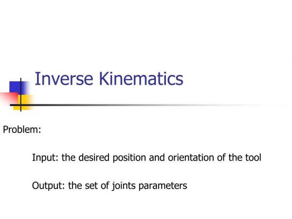
5. Forward vs. Inverse Kinematics Forward Kinematics Input: joint angles Output: link positions and orientations end effector position Inverse Kinematics Input: end effector Output: joint angles

6. Joints – relative movement • Every joint allowing motion in one dimension is said to have one degree of freedom (DOF) • Example: flying (Six DOF) • x, y, and z positions (prismatic or translation) • roll, pitch, and yaw (revolute or rotation)

7. Complex Joints

8. Hierarchical structure

9. Forward Kinematics: A Simple Example • Forward kinematics map as a coordinate transformation • The body local coordinate system of the end-effector was initially coincide with the global coordinate system • Forward kinematics map transforms the position and orientation of the end-effector according to joint angles Example from Jehee Lee

10. A Chain of Transformations

11. Thinking of Transformations • In a view of body-attached coordinate system

12. Thinking of Transformations • In a view of body-attached coordinate system

13. Thinking of Transformations • In a view of body-attached coordinate system

14. Thinking of Transformations • In a view of body-attached coordinate system

15. Thinking of Transformations • In a view of body-attached coordinate system

16. Thinking of Transformations • In a view of global coordinate system

17. Thinking of Transformations • In a view of global coordinate system

18. Thinking of Transformations • In a view of global coordinate system

19. Thinking of Transformations • In a view of global coordinate system

20. Thinking of Transformations • In a view of global coordinate system

21. Controlling forward kinematics • QWOP http://www.foddy.net/Athletics.html

22. IK solution uniqueness Zero One Two Many Images from http://freespace.virgin.net/hugo.elias/models/m_ik.htm

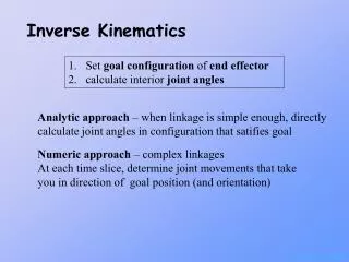
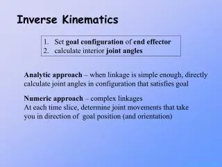
23. Inverse kinematics Given goal position for end effector Compute internal joint angles Simple linkages analytic solution Otherwise numeric iterative solution

24. Inverse kinematics – spaces Configuration space Reachable workspace

25. Analytic Inverse Kinematics • Given target position (X,Y) • Compute angle with respect to origin of linkage • Solve for angle of rotation for each joint • See reference text for solution and derivation

26. IK - numeric Solve iteratively – numerically solve for step toward goal Remember: a pose is the position and orientation of all links for given a set of joint angles - Compute the desired change from this pose Vector to the goal, or Minimal distance between end effector and goal - Compute set of changes to joint angles to make that change

27. IK math notation Given the values for each xi, we can compute each yi

28. IK – chain rule The change in output variables (y) relative to the change in input variables (x)

29. Inverse Kinematics - Jacobian Desired motion of end effector Unknown change in articulation variables The Jacobian is the matrix relating the two: describing how each coordinate changes with respect to each joint angle in our system

30. Inverse Kinematics - Jacobian Change in articulation variables Change in position Change in orientation Jacobian

31. Solving If J square, compute inverse, J-1 If J is not square, use of pseudo-inverse of Jacobian

32. IK – compute positional change vectors induced by changes in joint angles Instantaneous positional change vectors Desired change vector One approach to IK computes linear combination of change vectors that equal desired vector

33. IK - singularity Some singular configurations are not so easily recognizable

34. Inverse Kinematics - Numeric • Given • Current configuration • Goal position • Determine • Goal vector • Positions & local coordinate systems of interior joints (in global coordinates) Solve for change in joint angles & take small step – or clamp acceleration or clamp velocity • Repeat until: • Within epsilon of goal • Stuck in some configuration • Taking too long

35. IK – cyclic coordinate descent Heuristic solution Consider one joint at a time, from outside in At each joint, choose update that best gets end effector to goal position In 2D – pretty simple Goal axisi Ji EndEffector

36. Cyclic-Coordinate Descent - Starting with the root of our effector, R, to our current endpoint, E. - Next, we draw a vector from R to our desired endpoint, D - The inverse cosine of the dot product gives us the angle between the vectors: cos(a) = RD ● RE

37. Cyclic-Coordinate Descent Rotate our link so that RE falls on RD

38. Cyclic-Coordinate Descent Move one link up the chain, and repeat the process

39. Cyclic-Coordinate Descent The process is basically repeated until the root joint is reached. Then the process begins all over again starting with the end effector, and will continue until we are close enough to D for an acceptable solution.

40. Cyclic-Coordinate Descent

41. Cyclic-Coordinate Descent We’ve reached the root. Repeat the process

42. Cyclic-Coordinate Descent

43. Cyclic-Coordinate Descent

44. Cyclic-Coordinate Descent

45. Cyclic-Coordinate Descent

46. Cyclic-Coordinate Descent

47. Cyclic-Coordinate Descent We’ve reached the root again. Repeat the process until solution reached.

48. IK – cyclic coordinate descent Other orderings of processing joints are possible • Because of its procedural nature • Lends itself to enforcing joint limits • Easy to clamp angular velocity

49. IK – 3D cyclic coordinate descent Goal Projected goal axisi Ji EndEffector First – goal has to be projected onto plane defined by axis (normal to plane) and EF Second– determine angle at joint