Download
1 / 11
130 likes | 161 Views
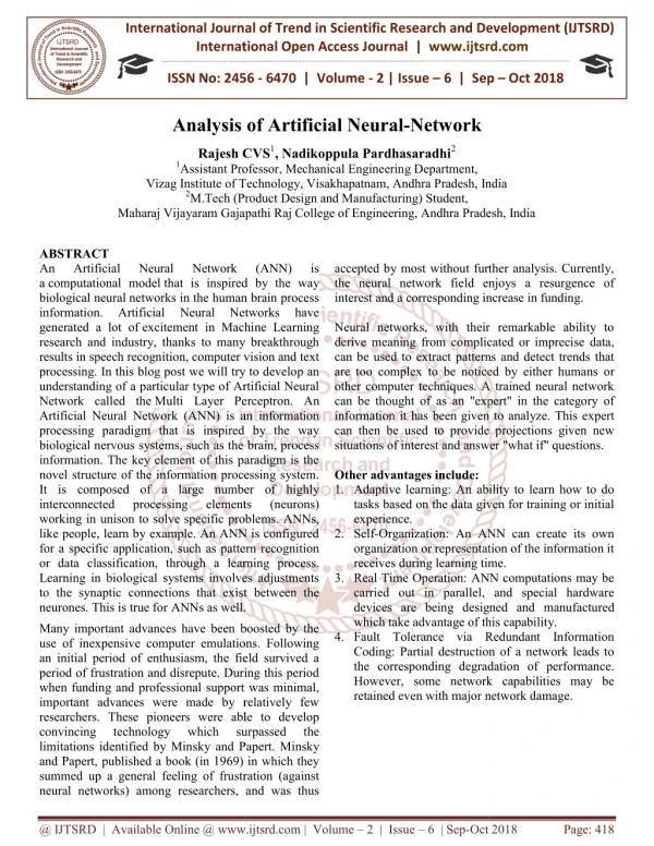
An Artificial Neural Network ANN is a computational model that is inspired by the way biological neural networks in the human brain process information. Artificial Neural Networks have generated a lot of excitement in Machine Learning research and industry, thanks to many breakthrough results in speech recognition, computer vision and text processing. In this blog post we will try to develop an understanding of a particular type of Artificial Neural Network called the Multi Layer Perceptron. An Artificial Neural Network ANN is an information processing paradigm that is inspired by the way biological nervous systems, such as the brain, process information. The key element of this paradigm is the novel structure of the information processing system. It is composed of a large number of highly interconnected processing elements neurons working in unison to solve specific problems. ANNs, like people, learn by example. An ANN is configured for a specific application, such as pattern recognition or data classification, through a learning process. Learning in biological systems involves adjustments to the synaptic connections that exist between the neurones. This is true for ANNs as well. Rajesh CVS | Nadikoppula Pardhasaradhi "Analysis of Artificial Neural-Network" Published in International Journal of Trend in Scientific Research and Development (ijtsrd), ISSN: 2456-6470, Volume-2 | Issue-6 , October 2018, URL: https://www.ijtsrd.com/papers/ijtsrd18482.pdf Paper URL: http://www.ijtsrd.com/engineering/mechanical-engineering/18482/analysis-of-artificial-neural-network/rajesh-cvs<br>

E N D
International Journal of Trend in International Open Access Journal International Open Access Journal | www.ijtsrd.com International Journal of Trend in Scientific Research and Development (IJTSRD) Research and Development (IJTSRD) www.ijtsrd.com ISSN No: 2456 ISSN No: 2456 - 6470 | Volume - 2 | Issue – 6 | Sep 6 | Sep – Oct 2018 Analysis o Analysis of Artificial Neural-Network Rajesh CVS1, Nadikoppula Pardhasaradhi2 Assistant Professor, Mechanical Engineering Department, Vizag Institute of Technology, Visakhapatnam, Andhra Pradesh, India M.Tech (Product Design and Manufacturing) Student, Maharaj Vijayaram Gajapathi Raj College of Engineering, Andhra Pradesh, India Maharaj Vijayaram Gajapathi Raj College of Engineering, Andhra Pradesh, India Rajesh C 1Assistant Professor Vizag Institute of Technology, Visakhapatnam, Andhra Pradesh, India 2M.Tech (Product Design and Ma Maharaj Vijayaram Gajapathi Raj College of Engineering, Andhra Pradesh, India Vizag Institute of Technology, Visakhapatnam, Andhra Pradesh, India accepted by most without further analysis. Currently, the neural network field enjoys a resurgence of interest and a corresponding increase in funding. Neural networks, with their remarkable ability to derive meaning from complicated or imprecise data, can be used to extract patterns and detect trends that are too complex to be noticed by either humans or other computer techniques. A trained neural network can be thought of as an "expert" in the category of information it has been given to analyze. This expert can then be used to provide projections given new situations of interest and answer "what if" questions. Other advantages include: 1.Adaptive learning: An ability to learn how to do tasks based on the data given for training or initial experience. 2.Self-Organization: An ANN can create its own organization or representation of the information it receives during learning time. 3.Real Time Operation: ANN computations may be carried out in parallel, and special hardware devices are being designed and manu which take advantage of this capability. 4.Fault Tolerance via Redundant Information Coding: Partial destruction of a network leads to the corresponding degradation of performance. However, some network capabilities may be retained even with major network damage. ABSTRACT An Artificial a computational model that is inspired by the way biological neural networks in the human brain process information. Artificial Neural generated a lot of excitement in Machine Learning research and industry, thanks to many breakthrough results in speech recognition, computer vision and text processing. In this blog post we will try to develop an understanding of a particular type of Artificial Neural Network called the Multi Layer Perceptron. Artificial Neural Network (ANN) is an information processing paradigm that is inspired by the way biological nervous systems, such as the brain, process information. The key element of this paradigm is the novel structure of the information processing system. It is composed of a large number of highly interconnected processing working in unison to solve specific problems. ANNs, like people, learn by example. An ANN is configured for a specific application, such as pattern recognition or data classification, through a learning process. Learning in biological systems involves adjustments to the synaptic connections that exist between the neurones. This is true for ANNs as well. ANNs as well. An Artificial Neural Neural Network Network (ANN) (ANN) is is accepted by most without further analysis. Currently, ld enjoys a resurgence of interest and a corresponding increase in funding. that is inspired by the way the human brain process Artificial Neural excitement in Machine Learning research and industry, thanks to many breakthrough results in speech recognition, computer vision and text In this blog post we will try to develop an understanding of a particular type of Artificial Neural Multi Layer Perceptron. An Artificial Neural Network (ANN) is an information processing paradigm that is inspired by the way nervous systems, such as the brain, process information. The key element of this paradigm is the novel structure of the information processing system. It is composed of a large number of highly interconnected processing to solve specific problems. ANNs, like people, learn by example. An ANN is configured for a specific application, such as pattern recognition or data classification, through a learning process. Learning in biological systems involves adjustments naptic connections that exist between the information. Networks Networks have have Neural networks, with their remarkable ability to derive meaning from complicated or imprecise data, can be used to extract patterns and detect trends that noticed by either humans or other computer techniques. A trained neural network can be thought of as an "expert" in the category of information it has been given to analyze. This expert can then be used to provide projections given new st and answer "what if" questions. Adaptive learning: An ability to learn how to do tasks based on the data given for training or initial elements elements (neurons) (neurons) Organization: An ANN can create its own organization or representation of the information it receives during learning time. Real Time Operation: ANN computations may be carried out in parallel, and special hardware devices are being designed and manufactured which take advantage of this capability. Fault Tolerance via Redundant Information Coding: Partial destruction of a network leads to the corresponding degradation of performance. However, some network capabilities may be network damage. Many important advances have been boosted by the use of inexpensive computer emulations. Following an initial period of enthusiasm, the field survived a period of frustration and disrepute. During this period when funding and professional support was minimal, important advances were made by relatively few researchers. These pioneers were able to develop convincing technology limitations identified by Minsky and Papert. Minsky and Papert, published a book (in 1969) in which they summed up a general feeling of frustration (against neural networks) among researchers, and was thus neural networks) among researchers, and was thus Many important advances have been boosted by the use of inexpensive computer emulations. Following an initial period of enthusiasm, the field survived a on and disrepute. During this period when funding and professional support was minimal, important advances were made by relatively few researchers. These pioneers were able to develop convincing technology which which ky and Papert. Minsky surpassed surpassed the the and Papert, published a book (in 1969) in which they summed up a general feeling of frustration (against @ IJTSRD | Available Online @ www.ijtsrd.com www.ijtsrd.com | Volume – 2 | Issue – 6 | Sep-Oct 2018 Oct 2018 Page: 418
International Journal of Trend in Scientific Research and Development (IJTSRD) ISSN: 2456 International Journal of Trend in Scientific Research and Development (IJTSRD) ISSN: 2456 International Journal of Trend in Scientific Research and Development (IJTSRD) ISSN: 2456-6470 elements (neurones) working in parallel to solve a specific problem. Neural networks learn by example. They cannot be programmed to perform a specific task. The examples must be selected carefully wasted or even worse the network might be functioning incorrectly. The disadvantage is that because the network finds out how to solve the problem by itself, its operation can elements (neurones) working in parallel to solve a specific problem. Neural networks learn by example. They cannot be programmed to perform a specific task. The examples must be selected carefully otherwise useful time is wasted or even worse the network might be functioning incorrectly. The disadvantage is that because the network finds out how to solve the problem by itself, its operation can be unpredictable. On the other hand, conventional computers use a cognitive approach to problem solving; the way the problem is to solved must be known and stated in small unambiguous instructions. These instructions are then converted to a high level language program and then into machine code that the computer can understand. These machines are totally predictable; if anything goes wrong is due to a software or hardware fault. Neural networks and conventional algorithmic computers are not in competition but complement each other. There are tasks are more suited to an algorithmic approach like arithmetic operations and tasks that are more suited to neural networks. Even more, a large number of tasks, require systems that use a combination of the two approaches (normally a conventional computer is used to supervise the neural network) in order to perform at maximum efficiency. Human and Artificial Neurones similarities Neural networks versus conventional computers Neural networks versus conventional computers On the other hand, conventional computers use a roach to problem solving; the way the problem is to solved must be known and stated in small unambiguous instructions. These instructions are then converted to a high level language program and then into machine code that the computer can machines are totally predictable; if anything goes wrong is due to a software or hardware Neural networks and conventional algorithmic computers are not in competition but complement each other. There are tasks are more suited to an proach like arithmetic operations and tasks that are more suited to neural networks. Even more, a large number of tasks, require systems that use a combination of the two approaches (normally a conventional computer is used to supervise the neural in order to perform at maximum efficiency. Human and Artificial Neurones - investigating the Neural networks take a different approach to problem solving than that of conventional computers. Conventional computers use an algorithmic approach i.e. the computer follows a set of instructions in order to solve a problem. Unless the specific steps that the computer needs to follow are known the computer cannot solve the problem. That restricts the problem solving capability of conventional computers to problems that we already understand and know how to solve. But computers would be so much more useful if they could do things that we don't exactly know how to do. Neural networks process information in a similar way the human brain does. The network is composed of a large number of highly interconnected processing highly interconnected processing Neural networks take a different approach to problem solving than that of conventional computers. Conventional computers use an algorithmic approach instructions in order to solve a problem. Unless the specific steps that the computer needs to follow are known the computer cannot solve the problem. That restricts the problem solving capability of conventional computers to rstand and know how to solve. But computers would be so much more useful if they could do things that we don't exactly Neural networks process information in a similar way the human brain does. The network is composed of a @ IJTSRD | Available Online @ www.ijtsrd.com www.ijtsrd.com | Volume – 2 | Issue – 6 | Sep-Oct 2018 Oct 2018 Page: 419
International Journal of Trend in Scientific Research and Development (IJTSRD) ISSN: 2456 International Journal of Trend in Scientific Research and Development (IJTSRD) ISSN: 2456 International Journal of Trend in Scientific Research and Development (IJTSRD) ISSN: 2456-6470 The synapse The synapse From Human Neurones to Artificial Neurones We conduct these neural networks by first trying to deduce the essential features of neurones and their interconnections. We then typically program a computer to simulate these features. However because our knowledge of neurones is incomplete and our computing power is limited, our models are necessarily gross idealizations of real networks of neurones. Some interesting numbers BRAIN From Human Neurones to Artificial Neurones We conduct these neural networks by first trying to ssential features of neurones and their interconnections. We then typically program a computer to simulate these features. However because our knowledge of neurones is incomplete and our computing power is limited, our models are tions of real networks of Some interesting numbers Much is still unknown about how the brain trains itself to process information, so theories abound. In the human brain, a typical neuron collects signals from others through a host of fine structures called dendrites. The neuron sends out spikes of electri activity through a long, thin stand known as an which splits into thousands of branches. At the end of each branch, a structure called a synapse activity from the axon into electrical effects that inhibit or excite activity from the axon into electrical effects that inhibit or excite activity in the connected neurones. When a neuron receives excitatory input that is sufficiently large compared with its inhibitory input, it sends a spike of electrical activity down its axon. Learning occurs by changing the effectiveness of the synapses so that the influence of one neuron on another changes. PC Much is still unknown about how the brain trains itself to process information, so theories abound. In the human brain, a typical neuron collects signals from others through a host of fine structures called . The neuron sends out spikes of electrical activity through a long, thin stand known as an axon, which splits into thousands of branches. At the end of Vprop=3*108 m/s 10 N=109 Vprop=100m/s 9 100 hz hz N N N=1010-1011 neurons The parallelism degree ~1014 1014processors with 100 Hz frequency. 104 connected at the same time. 14 like processors with 100 Hz connected at the synapse converts the activity from the axon into electrical effects that An engineering approach A neuron A more sophisticated neuron is the McCulloch and Pitts model (MCP). The difference from the previous model is that the inputs are ‘weighted’; the effect that each input has at decision making is dependent on the weight of the particular input. The weight o is a number which when multiplied with the input gives the weighted input. These weighted inputs are then added together and if they exceed a pre threshold value, the neuron fires. In any other case the neuron does not fire. axon into electrical effects that inhibit or excite activity in the connected neurones. When a neuron receives excitatory input that is sufficiently large compared with its inhibitory input, it sends a spike of electrical activity down its ccurs by changing the effectiveness of the synapses so that the influence of one neuron on A more sophisticated neuron is the McCulloch and Pitts model (MCP). The difference from the previous model is that the inputs are ‘weighted’; the effect that each input has at decision making is dependent on the weight of the particular input. The weight of an input is a number which when multiplied with the input gives the weighted input. These weighted inputs are then added together and if they exceed a pre-set threshold value, the neuron fires. In any other case the Components of a neuron @ IJTSRD | Available Online @ www.ijtsrd.com www.ijtsrd.com | Volume – 2 | Issue – 6 | Sep-Oct 2018 Oct 2018 Page: 420
International Journal of Trend in Scientific Research and Development (IJTSRD) ISSN: 2456 International Journal of Trend in Scientific Research and Development (IJTSRD) ISSN: 2456 International Journal of Trend in Scientific Research and Development (IJTSRD) ISSN: 2456-6470 In mathematical terms, the neuron fires if and only if; the addition of input weights and of the threshold makes this neuron a very flexible and powerful one. The MCP neuron has the ability to adapt to a particular situation by changing its weights and/or threshold. Various algorithms exist that cause the neuron to 'adapt'; the most used ones are the Delta rule and the back error propagation. The former is used in feed-forward networks and the latter in feedback networks. Architecture of neural networks Feed-forward networks Feed-forward ANNs allow signals to travel one way only; from input to output. There is no feedback (loops) i.e. the output of any layer does not affect that same layer. Feed-forward ANNs tend to be straight forward networks that associate inputs with outputs. They are extensively used in pattern recognition. This type of organization is also referred to as bottom down. Feedback networks Feedback networks (figure 1) can have signals traveling in both directions by introducing loops in the network. Feedback networks are very powerful and can get extremely complicated. Feedback networks are dynamic; their 'state' is changing continuously unt they reach an equilibrium point. They remain at the equilibrium point until the input changes and a new equilibrium needs to be found. Feedback architectures are also referred to as interactive or recurrent, although the latter term is often used to den feedback connections in single-layer organizations. Network layers The commonest type of artificial neural network consists of three groups, or layers, of units: a layer of "input" units is connected to a layer of " units, which is connected to a layer of "output The activity of the input units represents the raw information that is fed into the network. ical terms, the neuron fires if and only if; the addition of input weights and of the threshold makes this neuron a very flexible and powerful one. The MCP neuron has the ability to adapt to a particular situation by changing its weights and/or Various algorithms exist that cause the neuron to 'adapt'; the most used ones are the Delta rule and the back error propagation. The former is forward networks and the latter in The activity of each hidden unit is determined by the activities of the input units and the weights on the nput and the hidden units. The activity of each hidden unit is determined by the activities of the input units and the weights on the connections between the input and the hidden units. The behavior of the output units depends on the activity of the hidden units and the weights between the hidden and output units. This simple type of network is interesting because the hidden units are free to construct their representations of the input. The weights between the input and hidden units determine when each hidden unit is active, and so by modifying these weights, a hidden unit can choose what it represents. We also distinguish single architectures. The single-layer organization, in which all units are connected to one another, constitutes the most general case and is of more potential computational power than hierarchically structured multi-layer organizations. In multi units are often numbered by layer, instead of following a global numbering. Perceptrons The most influential work on neural nets in the 60's went under the heading 'perceptrons' a term coined by Frank Rosenblatt. The perceptron turns out to be an MCP model (neuron with weighted inputs) with some additional, fixed, pre processing. Units labeled A1, A2, Aj, Ap are called association units and their task is to extract specific, localized featured from the input images. Perceptrons mimic the basic idea behind the mammalian visual system. They were mainly used in pattern recognition even though their capabilities extended a lot more. The behavior of the output units depends on the activity of the hidden units and the weights between This simple type of network is interesting because the hidden units are free to construct their own representations of the input. The weights between the input and hidden units determine when each hidden unit is active, and so by modifying these weights, a hidden unit can choose what it represents. We also distinguish single-layer and multi-layer layer organization, in which all units are connected to one another, constitutes the most general case and is of more potential computational power than hierarchically structured layer organizations. In multi-layer networks, nits are often numbered by layer, instead of following a global numbering. with outputs. They are extensively used in pattern recognition. This type of organization is also referred to as bottom-up or top- The most influential work on under 'perceptrons' a term coined by Frank Rosenblatt. The the heading of of model (neuron with weighted inputs) with some additional, fixed, pre-- processing. Units labeled A1, A2, Aj, Ap are called association units and their task is to extract specific, localized featured from the input images. Perceptrons ehind the mammalian visual system. They were mainly used in pattern recognition even though their capabilities extended a lot more. Feedback networks are very powerful and can get extremely complicated. Feedback networks are dynamic; their 'state' is changing continuously until they reach an equilibrium point. They remain at the equilibrium point until the input changes and a new equilibrium needs to be found. Feedback architectures are also referred to as interactive or recurrent, although the latter term is often used to denote In Minsky and Papert wrote a book which described the limitations of single Perceptrons. 1969 layer organizations. in The commonest type of artificial neural network consists of three groups, or layers, of units: a layer of " units is connected to a layer of "hidden" they "output" units. layer The activity of the input units represents the raw at the book had was tremendous and caused a lot of neural network researchers to loose The impact that the book had was tremendous and caused a lot of neural network researchers to loose their interest. The book was very well written and their interest. The book was very well written and @ IJTSRD | Available Online @ www.ijtsrd.com www.ijtsrd.com | Volume – 2 | Issue – 6 | Sep-Oct 2018 Oct 2018 Page: 421
International Journal of Trend in Scientific Research and Development (IJTSRD) ISSN: 2456 International Journal of Trend in Scientific Research and Development (IJTSRD) ISSN: 2456 International Journal of Trend in Scientific Research and Development (IJTSRD) ISSN: 2456-6470 showed mathematically that single layer could not do some basic pattern recognition operations like determining the parity of a shape or determining whether a shape is connected or not. What they did not realize, until the 80's, is that given the appropriate training, multilevel perceptrons can do these operations. The Learning Process TYPES OF LEARNING All learning methods used for adaptive neural networks can be classified into two major categories: Supervised learning which incorporates an external teacher, so that each output unit is told what its desired response to input signals ought to be. During the learning process global information may be required. Paradigms of supervised learning include error-correction learning, learning and An important issue concerning supervised learning is the problem of error convergence, i.e. the minimization of error between the desired and computed unit values. The aim is to determine a set of weights which minimizes the error. One well method, which is common to many learning paradigms, is the least mean square (LMS) convergence. Unsupervised learning uses no external teacher and is based upon only local information. It is also referred to as self-organization, in the sense that it self-organizes data presented to the network and detects their emergent collective properties. Paradigms of unsupervised learning are Hebbian learning and competitive from Human Neurones to Artificial Ne aspect of learning concerns the distinction or not of a separate phase, during which the network is trained, and a subsequent operation phase. We say that a neural network learns off-line if the learning phase and the operation phase are distinct. A neural network learns on-line if it learns and operates at the same time. Usually, supervised learning is performed off line, whereas unsupervised learning is performed on line. single layer perceptrons TRANSFER FUNCTION The behavior of an ANN (Artificial Neural Network) depends on both the weights and the input function (transfer function) that is specified for the units. This function typically falls into one of three categories: linear (or ramp) threshold sigmoid f a 1 1 exp( For linear units, the output activity is proportional to the total weighted output. For threshold units, the output are set at one of two levels, depending on whether the total input is greater than or less than some threshold value. For sigmoid units, the output not linearly as the input changes. Sigmoid units bear a greater resemblance to real neurones than do linear or threshold units, but all three must be considered rough approximations. We can teach a three-layer network to perform a particular task by using the following procedure: We present the network with training examples, which consist of a pattern of activities for the input units together with the desired pattern of activities for the output units. We determine how closely t network matches the desired output. We change the weight of each connection so that the network produces a better approximation of the desired output. In order to train a neural network to perform some task, we must adjust the weights of each unit in such a way that the error between the desired output and the actual output is reduced. This process requires that the neural network compute the error derivative of the weights (EW). In other words, it must calculate how the error changes as each weight is increased or decreased slightly. The back propagation algorithm is the most widely used method for determining the EW. The back-propagation algorithm is easiest to understand if all the units in the network are linear. The algorithm computes each the EA, the rate at which the error changes as the , the rate at which the error changes as the could not do some basic pattern recognition ining the parity of a shape or determining whether a shape is connected or not. What they did not realize, until the 80's, is that given the appropriate training, multilevel perceptrons can do The behavior of an ANN (Artificial Neural Network) ends on both the weights and the input-output function (transfer function) that is specified for the units. This function typically falls into one of three exp( a ) d dt w , the output activity is proportional to the E w E , the output are set at one of two levels, depending on whether the total input is greater than or less than some threshold value. x w E E , , y y , x , w , the output varies continuously but not linearly as the input changes. Sigmoid units bear a greater resemblance to real neurones than do linear or threshold units, but all three must be considered rough told what its desired response to input signals ought to be. During the learning process global information may be required. Paradigms of supervised learning ning, reinforcement learning. learning. reinforcement learning An important issue concerning supervised learning is the problem of error convergence, i.e. the minimization of error between the desired and computed unit values. The aim is to determine a set of ts which minimizes the error. One well-known method, which is common to many learning paradigms, is the least mean square (LMS) and stochastic stochastic layer network to perform a particular task by using the following procedure: We present the network with training examples, which consist of a pattern of activities for the input units together with the desired pattern of activities for We determine how closely the actual output of the network matches the desired output. uses no external teacher and We change the weight of each connection so that the network produces a better approximation of the is based upon only local information. It is also organization, in the sense that it organizes data presented to the network and detects their emergent collective properties. In order to train a neural network to perform some weights of each unit in such a way that the error between the desired output and the actual output is reduced. This process requires that the neural network compute the error derivative of the ). In other words, it must calculate how hanges as each weight is increased or decreased slightly. The back propagation algorithm is the most widely used method for determining the Paradigms of unsupervised learning are Hebbian learning and competitive from Human Neurones to Artificial Neuron Esther aspect of learning concerns the distinction or not of a separate phase, during which the network is trained, and a subsequent operation phase. We say that a learning. learning. line if the learning phase ct. A neural network line if it learns and operates at the same time. Usually, supervised learning is performed off- line, whereas unsupervised learning is performed on- propagation algorithm is easiest to understand if all the units in the network are linear. hm computes each EW by first computing @ IJTSRD | Available Online @ www.ijtsrd.com www.ijtsrd.com | Volume – 2 | Issue – 6 | Sep-Oct 2018 Oct 2018 Page: 422
International Journal of Trend in Scientific Research and Development (IJTSRD) ISSN: 2456 International Journal of Trend in Scientific Research and Development (IJTSRD) ISSN: 2456 International Journal of Trend in Scientific Research and Development (IJTSRD) ISSN: 2456-6470 activity level of a unit is changed. For output units, the EA is simply the difference between the actual and the desired output. To compute the EA for a hidden unit in the layer just before the output layer, we first identify all the weights between that hidden unit and the output units to which it is connected. We then multiply those weights by the EAs of those output units and add the products. This sum equals the EA for the chosen hidden unit. After calculating all the EAs in the hidden layer just before the output layer, we can compute in like fashion the EAs for other layers, moving from layer to layer in a direction opposite to the way activities propagate through the network. This is what gives back propagation its name. Once the EA computed for a unit, it is straight forward to compute the EW for each incoming connection of the unit. The EW is the product of the EA and the activity through the incoming connection. Data filters That is all we need to know about Neural Nets, if we want to make forecasts. The next problem with which ZERO-PHASE FILTER The main equation of this filter: ) 1 ( ) 2 ( ) ( ) 1 ( ) ( n x b n x b n y The scheme of this filter activity level of a unit is changed. For output units, is simply the difference between the actual you will have to fight - is noise in real signals. And the biggest trouble, that nobody knows what is noise and what is pure signal. For example, how to choose the right variant problem right? ADAPTIVE FILTERS Main features, which we must obtain: 1.Zero-phase distortion (because we are going to make forecasts and we shouldn’t influence on the data’s phase we have. 2.We don’t know what real signal is and what is noise, especially in case of share values or smth like that. So one have to decide apriori what is the signal we want to obtain. In this chapter I’m going to make an overview of 3 types of adaptive filters: Zero filter), Kalman filter (error estimator), and Empirical mode decomposition. for in the the that hidden unit and the output units to which it is connected. We then multiply those weights by the s of those output units and add the products. This for the chosen hidden unit. After s in the hidden layer just before the output layer, we can compute in like fashion the s for other layers, moving from layer to layer in a direction opposite to the way activities propagate gh the network. This is what gives back Main features, which we must obtain: phase distortion (because we are going to make forecasts and we shouldn’t influence on the We don’t know what real signal is and what is noise, especially in case of share values or smth like that. So one have to decide apriori what is the EA has been computed for a unit, it is straight forward to compute for each incoming connection of the unit. The is the product of the EA and the activity through In this chapter I’m going to make an overview of 3 ers: Zero-phase filter (smoothing filter), Kalman filter (error estimator), and Empirical That is all we need to know about Neural Nets, if we want to make forecasts. The next problem with which ) 1 ) 1 ) 1 ... b ( nb nb x ( n nb ) ) 2 ( a y ( n ... a ( na y ( n na ) Where Z-1 – means that we take the previous value of the signal (moment (n-1)). b, a- are the filter coefficients. is the signal we have at the moment the signal we have at the momentn. means that we take the previous value of the Filter performs zero-phase digital filtering processing the input data in both the forward and reverse directions. After filtering in the forward direction, it reverses the filtered sequence and runs it back through the filter. The resulting sequence has precisely zero-phase distortion and double phase distortion and double the filter phase digital filtering by x (n ) processing the input data in both the forward and reverse directions. After filtering in the forward direction, it reverses the filtered sequence and runs it back through the filter. The resulting sequence has are the filter @ IJTSRD | Available Online @ www.ijtsrd.com www.ijtsrd.com | Volume – 2 | Issue – 6 | Sep-Oct 2018 Oct 2018 Page: 423
International Journal of Trend in Scientific Research and Development (IJTSRD) ISSN: 2456 International Journal of Trend in Scientific Research and Development (IJTSRD) ISSN: 2456 International Journal of Trend in Scientific Research and Development (IJTSRD) ISSN: 2456-6470 order. filter minimizes start-up and ending transients by matching initial conditions, and works for both real and complex inputs. Note that filter should not be used with differentiator and Hilbert FIR filters, since the operation of these filters depends heavily on their phase response. up and ending transients coefficient are very good. It means that it’s is possible to use this filter, but with some kind of error coefficient are very good. It means that it to use this filter, but with some kind of error estimator. KALMAN FILTER (ERROR Consider a linear, discrete-time dynamical system. The concept of state is fundamental to this description. The state vector or simply state, denoted by x, is defined as the minimal set of data that is sufficient to uniquely describe the unforced dynamical behavior of the system; the subscript n denotes discrete time. In other words, the state is the least amount of data on the past behavior of the sys is needed to predict its future behavior. Typically, the state xk is unknown. To estimate it, we use a set of observed data, denoted by the vector y mathematical terms, the block diagram embodies the following pair of equations: by matching initial conditions, and works for both real and complex inputs. Note that filter should not be used with differentiator and Hilbert FIR filters, since ers depends heavily on their KALMAN FILTER (ERROR ESTIMATOR) time dynamical system. The concept of state is fundamental to this description. The state vector or simply state, denoted by x, is defined as the minimal set of data that is sufficient to uniquely describe the unforced dynamical behavior of the system; the subscript n denotes discrete time. In other words, the state is the least amount of data on the past behavior of the system that is needed to predict its future behavior. Typically, the is unknown. To estimate it, we use a set of observed data, denoted by the vector yk. In mathematical terms, the block diagram embodies the Problem: After the neural net the forecast will have 1 day delay if we tried to make forecast for one day. It looks like the picture on the right. But I should mention that all statistical values e.g. correlation mention that all statistical values e.g. correlation Problem: After the neural net the forecast will have 1 day delay if we tried to make forecast for one day. It looks like the picture on the right. But I should The equation of this filter is given below: k n x a n x The equation of this filter is given below: x ) 1 cx ) 1 net ) 1 ( ) ( ( n )[ y y ( n ) ac ( n 1 1 n )], where x ( n ) ax ( n w ( n model of generating generating signal , w Problem: After Kalman filter the error became less, but there is still a day delay. The solution is Empirical Mode Decomposition. EMPIRICAL MODE DECOMPOSITION A new nonlinear technique, referred to as Mode Decomposition (EMD), has recently been pioneered by N.E. Huang et al. for adaptively representing nonstationary signals as sums of zero mean AMFM components [2]. Although it often proved remarkably effective [1, 2, 5, 6, 8], the technique is faced with the difficulty of being essentially defined by an algorithm, and therefor not admitting an analytical formulation which would allow for a theoretical analysis and performance evaluation. The purpose of this paper is therefore to contribute experimentally to a better understanding of contribute experimentally to a better understanding of ( n ) white noise and ( n ) ( n ) ( ) signal after neural , ( n ) white noise Problem: After Kalman filter the error became less, but there is still a day delay. The solution is Empirical Problem: After Kalman filter the error became less, but there is still a day delay. The solution is Empirical the method and to propose various upon the original formulation. Some preliminary elements of experimental performance evaluation will also be provided for giving a flavor of the efficiency of the decomposition, as well as of the difficulty of its interpretation. The starting point of Decomposition (EMD) is to consider oscillations in signals at a very local level. In fact, if we look at the evolution of a signal x(t) between two consecutive extrema (say, two minima occurring at times extrema (say, two minima occurring at times t− and POSITION A new nonlinear technique, referred to as Empirical (EMD), has recently been the method and to propose various improvements upon the original formulation. Some preliminary elements of experimental performance evaluation will also be provided for giving a flavor of the efficiency of the decomposition, as well as of the difficulty of its for adaptively representing nonstationary signals as sums of zero- mean AMFM components [2]. Although it often proved remarkably effective [1, 2, 5, 6, 8], the technique is faced with the difficulty of being essentially defined by an algorithm, and therefore of not admitting an analytical formulation which would allow for a theoretical analysis and performance evaluation. The purpose of this paper is therefore to point of the the Empirical Empirical Mode Mode Decomposition (EMD) is to consider oscillations in signals at a very local level. In fact, if we look at the ) between two consecutive @ IJTSRD | Available Online @ www.ijtsrd.com www.ijtsrd.com | Volume – 2 | Issue – 6 | Sep-Oct 2018 Oct 2018 Page: 424
International Journal of Trend in Scientific Research and Development (IJTSRD) ISSN: 2456 International Journal of Trend in Scientific Research and Development (IJTSRD) ISSN: 2456 International Journal of Trend in Scientific Research and Development (IJTSRD) ISSN: 2456-6470 t+), we can heuristically define a (local) high frequency part {d(t), t− ≤ t ≤ t+}, or local which corresponds to the oscillation terminating at the two minima and passing through the maximum which necessarily exists in between them. For the picture to be complete, one still has to identify the corresponding (local) low-frequency part local trend, so that we have x(t) = m(t) + ≤ t+. Assuming that this is done in some proper way for all the oscillations composing the entire signal, the procedure can then be applied on the residual consisting of all local trends, and constitutive components of a signal can therefore be iteratively extracted. Given a signal x(t), the effective algorithm of EMD can be summarized as follows: 1.Identity all extrema of x(t) 2.Interpolate between minima (resp. maxima), ending up with some envelope emax(t)) 3.Compute the mean m(t) = (emin(t)+e 4.Extract the detail d(t) = x(t) − m(t) 5.Iterate on the residual m(t) In practice, the above procedure has to be refined by a sifting process which amounts to first iterating steps 1 to 4 upon the detail signal d(t), until this latter can be considered as zero-mean according to some stopping criterion. Once this is achieved, the detail is referred to as an Intrinsic Mode Function corresponding residual is computed and step 5 applies. By construction, the number of extrema is decreased when going from one residual to the next, and the whole decomposition is guaranteed to be completed with a finite number of modes. Modes and residuals have been heuristically introduced on “spectral” arguments, but this must not be considered from a too narrow perspective. First, it is worth stressing the fact that, even in the case of harmonic oscillations, the high vs. low frequency discrimination mentioned above applies only locally and corresponds by no way to a pre-determined sub band filtering (as, e.g., in a wavelet transform). Selection of modes rather corresponds to an automatic and adaptive (signal-dependent) time-variant filtering. Let’s try to do this procedure with next signal 400 sin( 5 , 0 ) 20 sin( 7 , 0 t x istically define a (local) high- , or local detail, IMF#1 IMF#1 which corresponds to the oscillation terminating at the two minima and passing through the maximum which necessarily exists in between them. For the picture to , one still has to identify the frequency part m(t), or ) + d(t) for t− ≤ t +. Assuming that this is done in some proper way for all the oscillations composing the entire signal, the dure can then be applied on the residual consisting of all local trends, and constitutive components of a signal can therefore be iteratively IMF#2 IMF#2 ), the effective algorithm Interpolate between minima (resp. maxima), ending up with some envelope emin(t) (resp. emax(t))/2 In practice, the above procedure has to be refined by a process which amounts to first iterating steps 1 ), until this latter can be mean according to some stopping Let’s try to filter from high frequency part (light gray Let’s try to filter from high frequency part (light gray – EMD, dark gray – zero phase filters) zero phase filters) criterion. Once this is achieved, the detail is referred Intrinsic Mode Function (IMF), the corresponding residual is computed and step 5 number of extrema is decreased when going from one residual to the next, and the whole decomposition is guaranteed to be completed with a finite number of modes. Modes and residuals have been heuristically introduced on not be considered from a too narrow perspective. First, it is worth stressing the fact that, even in the case of harmonic oscillations, the high vs. low frequency discrimination Problem: Using this method we have strong boundary effects. Sifting process can minimize this effect, but not at all. ZERO-PHASE FILTER +KALMAN +EMD = SOLUTION The so called solution is next. We should use data, obtained from zero-phase filter on should use linear weighed sum of zero some IMF’s in the middle. And after the forecast is done, we should apply Kalman filter to the forecast. Let’s try to do that. The figure on the bottom is the forecast of some company’s sh set). There is no delay. Problem: Using this method we have strong boundary effects. Sifting process can minimize this effect, but and corresponds ined sub band filtering (as, e.g., in a wavelet transform). Selection of modes rather corresponds to an automatic and adaptive variant filtering. Let’s try to do this procedure with next signal PHASE FILTER +KALMAN FILTER The so called solution is next. We should use data, phase filter on the boundaries, we should use linear weighed sum of zero-phase and some IMF’s in the middle. And after the forecast is done, we should apply Kalman filter to the forecast. Let’s try to do that. The figure on the bottom is the forecast of some company’s share value (production 01 01 t ), t [ ] ] @ IJTSRD | Available Online @ www.ijtsrd.com www.ijtsrd.com | Volume – 2 | Issue – 6 | Sep-Oct 2018 Oct 2018 Page: 425
International Journal of Trend in Scientific Research and Development (IJTSRD) ISSN: 2456 International Journal of Trend in Scientific Research and Development (IJTSRD) ISSN: 2456 International Journal of Trend in Scientific Research and Development (IJTSRD) ISSN: 2456-6470 The bottom figures are zoomed pictures of previous figure The bottom figures are zoomed pictures of previous HOLDER-FUNCTION IMPORTANT The main idea is next. Consider derived, that | ) ( ) ( | t f t t f that we means 0 So this formula is a somewhat connection between “bad” functions and “good” functions. If we will look on this formula with more precise we will notice, that we can catch moments in time, when our function knows, that it’s going to change it’s behavior from one to another. It means that today we can make a forecast on tomorrow behavior. But one should mention that we don’t know the sigh on what behavior is going to change. FUNCTION BEHAVIOR BEHAVIOR IS IS The main idea is next. Consider Holder f ( t ) D f break break t of ] 1 , 0 [ second ( ) const have ( O t ) , ( t ) order 1 means that we have ( t t ) So this formula is a somewhat connection between “bad” functions and “good” functions. If we will look on this formula with more precise we will notice, that we can catch moments in time, when our function hange it’s behavior from one to another. It means that today we can make a forecast on tomorrow behavior. But one should mention that we don’t know the sigh on what The figure on the bottom is the result of mat lab program which shows all results in one window. the result of mat lab program which shows all results in one window. the result of mat lab program which shows all results in one window. @ IJTSRD | Available Online @ www.ijtsrd.com www.ijtsrd.com | Volume – 2 | Issue – 6 | Sep-Oct 2018 Oct 2018 Page: 426
International Journal of Trend in Scientific Research and Development (IJTSRD) ISSN: 2456 International Journal of Trend in Scientific Research and Development (IJTSRD) ISSN: 2456 International Journal of Trend in Scientific Research and Development (IJTSRD) ISSN: 2456-6470 And pay attention to field Holder after filtration was done And pay attention to field Holder after filtration was done So we can make forecasts without delay and we (In case of IMF filtering Holder function is (In case of IMF filtering Holder function is smoother) So we can make forecasts without delay and we know Horst behavior. know Horst behavior. RESULTS If you are going to make forecast, you will need filters. The best way to make forecast is to use adaptive filters. Three of them I showed you. The thing I will show next isn’t the best way to make forecasts. I’m going to teach ANN to make forecast for one day. After that we suggest predicted value as an input to make forecast for the second day and so on. Let’s try to make forecast for Siemens share values. Here is Siemens function (for share values) Here is Siemens function (for share values) If you are going to make forecast, you will need filters. The best way to make forecast is to use adaptive filters. Three of them I showed you. The thing I will show next isn’t the best way to make forecasts. I’m going to teach forecast for one day. After that we suggest predicted value as an input to make forecast for the If you are going to make forecast, you will need filters. The best way to make forecast is to use adaptive filters. Three of them I showed you. The thing I will show next isn’t the best way to make forecasts. I’m going to teach forecast for one day. After that we suggest predicted value as an input to make forecast for the second day and so on. Let’s try to make forecast for Siemens share values. Let’s filter it. Now we are ready to make forecast. Here is the forecast in comparison with real data. Here is the forecast in comparison with real data. @ IJTSRD | Available Online @ www.ijtsrd.com www.ijtsrd.com | Volume – 2 | Issue – 6 | Sep-Oct 2018 Oct 2018 Page: 427
International Journal of Trend in Scientific Research and Development (IJTSRD) ISSN: 2456 International Journal of Trend in Scientific Research and Development (IJTSRD) ISSN: 2456 International Journal of Trend in Scientific Research and Development (IJTSRD) ISSN: 2456-6470 3,165 3,16 3,155 3,15 3,145 forecast real 3,14 3,135 3,13 3,125 3,12 3,115 0 2 4 6 8 10 12 14 Of course it’s is better to use another techniques to make forecast’s for few days. But this approach can give you a chance to make forecast for 5 REFERENCE 1.Web-Site made by Christos Stergiou and Dimitrios Siganos http://www.doc.ic.ac.uk http://www.doc.ic.ac.uk Of course it’s is better to use another techniques to make forecast’s for few days. But this approach can give Of course it’s is better to use another techniques to make forecast’s for few days. But this approach can give you a chance to make forecast for 5-6 days depending on the function you are working with. depending on the function you are working with. Site made by Christos Stergiou and 6.Gabriel Rilling, Patrick Flandrin and Paulo Goncalves “On Empirical Mode Decomposition and its algorithms” Gabriel Rilling, Patrick Flandrin and Paulo Goncalves “On Empirical Mode Decomposition 2.S. A. Shumsky “Selected lections about neural computing” A. Shumsky “Selected lections about neural 7.Norden E. Huang1, Zheng Shen, Steven R. Long, Manli C. Wu, Hsing H. Shih, Quanan Zheng, Nai Chyuan Yen, Chi Chao Tung and Henry H. Liu “The empirical mode decomposition and the Hilbert spectrum for nonlinear and non time series analysis” Norden E. Huang1, Zheng Shen, Steven R. Long, Wu, Hsing H. Shih, Quanan Zheng, Nai- Chyuan Yen, Chi Chao Tung and Henry H. Liu “The empirical mode decomposition and the Hilbert spectrum for nonlinear and non-stationary 3.Simon Haykin “Kalman Filtering and Neural Networks” Copyright © 2001 John Wiley & Sons, Inc. ISBNs: 0-471-36998-5 (Hardback); 0 22154-6 (Electronic) “Kalman Filtering and Neural Networks” Copyright © 2001 John Wiley & Sons, 5 (Hardback); 0-471- 4.Web-Site made by Base Group Labs © 1995 http://www.basegroup.ru Group Labs © 1995-2006 8.Gabriel Rilling, Patrick Flandrin and Paulo Goncalves “Detrending Empirical Mode Decompositions” ecompositions” Gabriel Rilling, Patrick Flandrin and Paulo ding and denoising with 5.Vesselin Vatchev, USC November 20, 2002, “The analysis of the Empirical Mode Decomposition Method ” Vatchev, USC November 20, 2002, “The analysis of the Empirical Mode Decomposition @ IJTSRD | Available Online @ www.ijtsrd.com www.ijtsrd.com | Volume – 2 | Issue – 6 | Sep-Oct 2018 Oct 2018 Page: 428