Download

1 / 45
550 likes | 1.2k Views
Artificial Neural Network Supervised Learning. دكترمحسن كاهاني http://www.um.ac.ir/~kahani/. Back-propagation neural network. Learning in a multilayer network proceeds the same way as for a perceptron. A training set of input patterns is presented to the network.

E N D
Artificial Neural Network Supervised Learning دكترمحسن كاهاني http://www.um.ac.ir/~kahani/
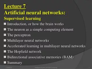
Back-propagation neural network • Learning in a multilayer network proceeds the same way as for a perceptron. • A training set of input patterns is presented to the network. • The network computes its output pattern, and if there is an error - or in other words a difference between actual and desired output patterns - the weights are adjusted to reduce this error. سيستمهاي خبره و مهندسي دانش-دكتر كاهاني
BP Training Phases • In a back-propagation neural network, the learning algorithm has two phases. • A training input pattern is presented to the network input layer. The network propagates the input pattern from layer to layer until the output pattern is generated by the output layer. • If this pattern is different from the desired output, an error is calculated and then propagated backwards through the network from the output layer to the input layer. The weights are modified as the error is propagated. سيستمهاي خبره و مهندسي دانش-دكتر كاهاني
Three-layer BP network سيستمهاي خبره و مهندسي دانش-دكتر كاهاني
The back-propagation training algorithm • Step 1: Initialisation • Set all the weights and threshold levels of the network to random numbers uniformly distributed inside a small range: where Fi is the total number of inputs of neuron i in the network. • The weight initialization is done on a neuron-by-neuron basis. سيستمهاي خبره و مهندسي دانش-دكتر كاهاني
Step 2: Activation • Activate the BP network by applying: • inputs x1(p), x2(p),…, xn(p) • desired outputs yd,1(p), yd,2(p),…, yd,n(p). (a) Calculate the actual outputs of the neurons in the hidden layer: where n is the number of inputs of neuron j in the hidden layer, and sigmoid is the sigmoid activation function. سيستمهاي خبره و مهندسي دانش-دكتر كاهاني
Step 2: Activation (cont.) (b) Calculate the actual outputs of the neurons in the output layer: where m is the number of inputs of neuron k in the output layer. سيستمهاي خبره و مهندسي دانش-دكتر كاهاني
Step 3: Weight training • Update the weights in the BP network propagating backward the errors associated with output neurons. (a) Calculate the error gradient for the neurons in the output layer: d k ( p) = yk ( p) .[1- yk ( p)]. ek ( p) where ek ( p) = yd ,k ( p) - yk ( p) Calculate the weight corrections: Dwjk ( p) =a . y j ( p) .d k ( p) Update the weights at the output neurons: wjk ( p +1) = wjk ( p) + Dwjk ( p) سيستمهاي خبره و مهندسي دانش-دكتر كاهاني
Step 3: Weight training (cont.) (b) Calculate the error gradient for the neurons in the hidden layer: Calculate the weight corrections: Dwij ( p) =a . xi ( p) .d j ( p) Update the weights at the hidden neurons: wij ( p +1) = wij ( p) + Dwij ( p) سيستمهاي خبره و مهندسي دانش-دكتر كاهاني
Step 4: Iteration • Increase iteration p by one, go back to Step 2 and repeat the process until the selected error criterion is satisfied. سيستمهاي خبره و مهندسي دانش-دكتر كاهاني
Example Three-layer network for solving the Exclusive-OR operation سيستمهاي خبره و مهندسي دانش-دكتر كاهاني
Example (cont.) • The effect of the threshold applied to a neuron in the hidden or output layer is represented by its weight, q, connected to a fixed input equal to -1. • The initial weights and threshold levels are set randomly as follows: w13 = 0.5, w14 = 0.9, w23 = 0.4, w24 = 1.0, w35 = -1.2, w45 = 1.1 q3 = 0.8, q4 = -0.1 and q5 = 0.3. سيستمهاي خبره و مهندسي دانش-دكتر كاهاني
Example (cont.) • We consider a training set where inputs x1 and x2 are equal to 1 and desired output yd,5 is 0. The actual outputs of neurons 3 and 4 in the hidden layer are calculated as • Now the actual output of neuron 5 in the output layer is determined as: • Thus, the following error is obtained: e = yd,5- y5 = 0 - 0.5097 = -0.5097 سيستمهاي خبره و مهندسي دانش-دكتر كاهاني
Example (cont.) • The next step is weight training. To update the weights and threshold levels in our network, we propagate the error, e, from the output layer backward to the input layer. • First, we calculate the error gradient for neuron 5 in the output layer: d5= y5 (1- y5) e = 0.5097 .(1- 0.5097) . (-0.5097) = -0.1274 • Then we determine the weight corrections assuming that the learning rate parameter, a, is equal to 0.1: سيستمهاي خبره و مهندسي دانش-دكتر كاهاني
Example (cont.) • Next we calculate the error gradients for neurons 3 and 4 in the hidden layer: • We then determine the weight corrections: سيستمهاي خبره و مهندسي دانش-دكتر كاهاني
Example (cont.) • At last, we update all weights and threshold: w13 = w13 + Dw13 = 0.5 + 0.0038 = 0.5038 w14 = w14 + Dw14 = 0.9 - 0.0015 = 0.8985 w23 = w23 + Dw23 = 0.4 + 0.0038 = 0.4038 w24 = w24 + Dw24 = 1.0 - 0.0015 = 0.9985 w35 = w35 + Dw35 = -1.2 - 0.0067 = -1.2067 w45 = w45 + Dw45 = 1.1- 0.0112 = 1.0888 q3 = q3 + Dq3 = 0.8 - 0.0038 = 0.7962 q4 = q4 + Dq4 = -0.1 + 0.0015 = -0.0985 q5 = q5 + Dq5 = 0.3 + 0.0127 = 0.3127 • The training process is repeated until the sum of squared errors is less than 0.001. سيستمهاي خبره و مهندسي دانش-دكتر كاهاني
Learning curve for Exclusive-OR سيستمهاي خبره و مهندسي دانش-دكتر كاهاني
Final results of learning سيستمهاي خبره و مهندسي دانش-دكتر كاهاني
McCulloch-Pitts model for solving the Exclusive-OR سيستمهاي خبره و مهندسي دانش-دكتر كاهاني
Decision boundaries • (a) Decision boundary constructed by hidden neuron 3; • (b) Decision boundary constructed by hidden neuron 4; • (c) Decision boundaries constructed by the complete three-layer network سيستمهاي خبره و مهندسي دانش-دكتر كاهاني
Accelerated learning in multilayer neural networks • A multilayer network learns much faster when the sigmoidal activation function is represented by a hyperbolic tangent: where a and b are constants. • Suitable values for a and b are: a = 1.716 and b = 0.667 سيستمهاي خبره و مهندسي دانش-دكتر كاهاني
Accelerated learning (cont.) • We also can accelerate training by including a momentum term in the delta rule: Dwjk ( p) = b .Dwjk ( p -1) +a . y j ( p) . dk ( p) • where b is a positive number (0 ≤ b < 1) called the momentum constant. Typically, the momentum constant is set to 0.95. • This equation is called the generalised delta rule. سيستمهاي خبره و مهندسي دانش-دكتر كاهاني
Learning with momentum for operation Exclusive-OR سيستمهاي خبره و مهندسي دانش-دكتر كاهاني
Learning with adaptive learning rate • To accelerate the convergence and yet avoid the danger of instability, we can apply two heuristics: Heuristic 1 • If the change of the sum of squared errors has the same algebraic sign for several consequent epochs, then the learning rate parameter, a, should be increased. Heuristic 2 • If the algebraic sign of the change of the sum of squared errors alternates for several consequent epochs, then the learning rate parameter, a, should be decreased. سيستمهاي خبره و مهندسي دانش-دكتر كاهاني
Learning with adaptive learning rate (cont.) • Adapting the learning rate requires some changes in the back-propagation algorithm. • If the sum of squared errors at the current epoch exceeds the previous value by more than a predefined ratio (typically 1.04), the learning rate parameter is decreased (typically y multiplying by 0.7) and new weights and thresholds are calculated. • If the error is less than the previous one, the learning rate is increased (typically by multiplying by 1.05). سيستمهاي خبره و مهندسي دانش-دكتر كاهاني
Learning with adaptive learning rate (cont.) سيستمهاي خبره و مهندسي دانش-دكتر كاهاني
Learning with momentum and adaptive learning rate سيستمهاي خبره و مهندسي دانش-دكتر كاهاني
The Hopfield Network • The brain’s memory, however, works by association. • For example, we can recognize a familiar face even in an unfamiliar environment within 100-200 ms. • BPN is good for pattern recognition problems. • we need a recurrent neural network. • A recurrent neural network has feedback loops from its outputs to its inputs. • The stability of recurrent networks was solved only in 1982, when John Hopfield formulated the physical principle of storing information in a dynamically stable network. سيستمهاي خبره و مهندسي دانش-دكتر كاهاني
Single-layer n-neuron Hopfield network سيستمهاي خبره و مهندسي دانش-دكتر كاهاني
z-1 z-1 z-1 MultiLayer Hopfield Network input hidden output سيستمهاي خبره و مهندسي دانش-دكتر كاهاني
Hopfield Network Attributes • The Hopfield network uses McCulloch and Pitts neurons with the sign activation function as its computing element: سيستمهاي خبره و مهندسي دانش-دكتر كاهاني
Hopfield Network Attributes • The current state of the Hopfield network is determined by the current outputs of all neurons, y1, y2, . . ., yn. Thus, for a single-layer n-neuron network, the state can be defined by the state vector as: سيستمهاي خبره و مهندسي دانش-دكتر كاهاني
Hopfield Network Attributes • In the Hopfield network, synaptic weights between neurons are usually represented in matrix form as follows: where Mis the number of states to be memorized by the network, Ymis the n-dimensional binary vector, Iis n × n identity matrix, and superscript T denotes a matrix transposition. سيستمهاي خبره و مهندسي دانش-دكتر كاهاني
Possible states for the three-neuron Hopfield network سيستمهاي خبره و مهندسي دانش-دكتر كاهاني
CalculationnetworkHopfield • The stable state-vertex is determined by the weight matrix W, the current input vector X, and the threshold matrix • If the input vector is partially incorrect or incomplete, the initial state will converge into the stable state-vertex after a few iterations. سيستمهاي خبره و مهندسي دانش-دكتر كاهاني
Hopfield Network Calculations (Cont.) • Suppose, for instance, that our network is required to memorize two opposite states, (1, 1, 1) and (-1, -1, -1). Thus, or where Y1 and Y2 are the three-dimensional vectors. • The 3 x3 identity matrix I is سيستمهاي خبره و مهندسي دانش-دكتر كاهاني
Hopfield Network Calculations (Cont.) • Thus, we can now determine the weight matrix as follows: • Next, the network is tested by the sequence of input vectors, X1 and X2, which are equal to the output (or target) vectors Y1 and Y2, respectively. سيستمهاي خبره و مهندسي دانش-دكتر كاهاني
Hopfield Network Calculations (Cont.) • First, we activate the Hopfield network by applying the input vector X. Then, we calculate the actual output vector Y, and finally, we compare the result with the initial input vector X. سيستمهاي خبره و مهندسي دانش-دكتر كاهاني
Hopfield Network Calculations (Cont.) • The remaining six states are all unstable. However, stable states (also called fundamental memories) are capable of attracting states that are close to them. • The fundamental memory (1, 1, 1) attracts unstable states (-1, 1, 1), (1, -1, 1) and (1, 1, -1). Each of these unstable states represents a single error, compared to the fundamental memory (1, 1, 1). • The fundamental memory (-1, -1, -1) attracts unstable states (-1, -1, 1), (-1, 1, -1) and (1, -1, -1). • Thus, the Hopfield network can act as an error correction network. سيستمهاي خبره و مهندسي دانش-دكتر كاهاني
Storage capacity of the Hopfield network • Storage capacity is the largest number of fundamental memories that can be stored and retrieved correctly. • The maximum number of fundamental memories Mmax that can be stored in the n-neuron recurrent network is limited by Mmax= 0.15 n سيستمهاي خبره و مهندسي دانش-دكتر كاهاني
Bidirectional associative memory (BAM) • The Hopfield network: autoassociative memory • It can retrieve a corrupted or incomplete memory • but cannot associate this memory with another different memory. • Human memory is essentially associative. • Associative memory needs a recurrent neural network capable of accepting an input pattern on one set of neurons and producing a related, but different, output pattern on another set of neurons. سيستمهاي خبره و مهندسي دانش-دكتر كاهاني
Bidirectional associative memory (BAM) • Bidirectional associative memory (BAM), first proposed by Bart Kosko, is a heteroassociative network. • It associates patterns from one set, set A, to patterns from another set, set B, and vice versa. • Like a Hopfield network, the BAM can generalize and also produce correct outputs despite corrupted or incomplete inputs. سيستمهاي خبره و مهندسي دانش-دكتر كاهاني
BAM operation سيستمهاي خبره و مهندسي دانش-دكتر كاهاني
BAM Concept • The basic idea behind the BAM is to store pattern pairs so that when n-dimensional vector X from set A is presented as input, the BAM recalls m-dimensional vector Y from set B, but when Y is presented as input, the BAM recalls X. • To develop the BAM, we need to create a correlation matrix for each pattern pair we want to store. • BAM weight matrix: • where M is the number of pattern pairs to be stored in the BAM. سيستمهاي خبره و مهندسي دانش-دكتر كاهاني
Stability and storage capacity of the BAM • The BAM is unconditionally stable. This means that any set of associations can be learned without risk of instability. Max. no. of associations < No. of neurons in the smaller layer. • The more serious problem with the BAM is incorrect convergence. The BAM may not always produce the closest association. In fact, a stable association may be only slightly related to the initial input vector. سيستمهاي خبره و مهندسي دانش-دكتر كاهاني