Download
1 / 7
70 likes | 73 Views
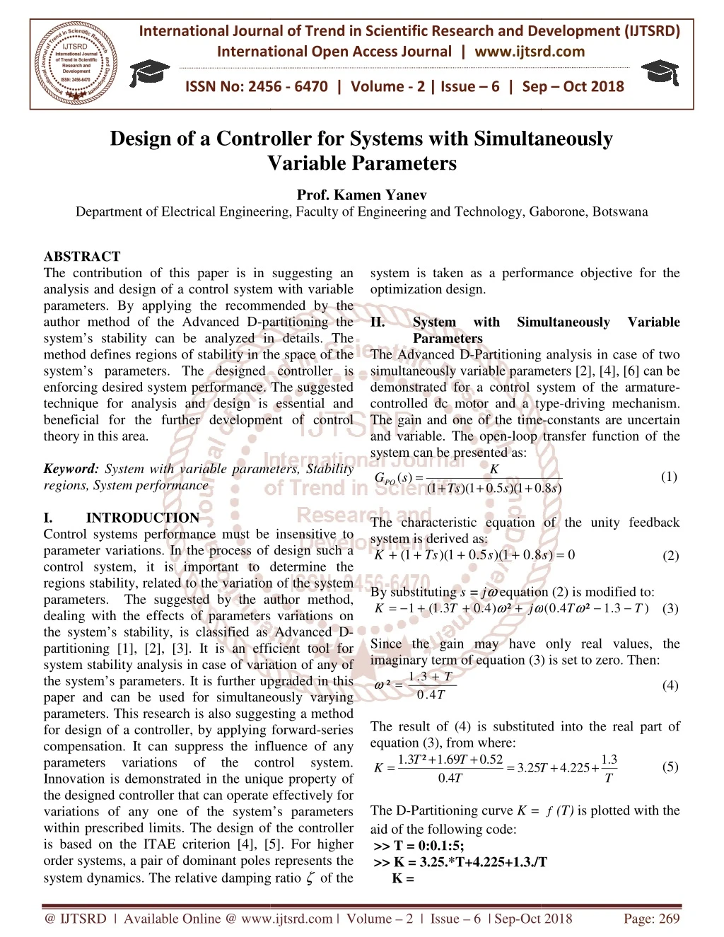
The contribution of this paper is in suggesting an analysis and design of a control system with variable parameters. By applying the recommended by the author method of the Advanced D partitioning the system's stability can be analyzed in details. The method defines regions of stability in the space of the system's parameters. The designed controller is enforcing desired system performance. The suggested technique for analysis and design is essential and beneficial for the further development of control theory in this area. Prof. Kamen Yanev "Design of a Controller for Systems with Simultaneously Variable Parameters" Published in International Journal of Trend in Scientific Research and Development (ijtsrd), ISSN: 2456-6470, Volume-2 | Issue-6 , October 2018, URL: https://www.ijtsrd.com/papers/ijtsrd18440.pdf Paper URL: http://www.ijtsrd.com/engineering/electrical-engineering/18440/design-of-a-controller-for-systems-with-simultaneously-variable-parameters/prof-kamen-yanev<br>

E N D
International Journal of Trend in International Open Access Journal International Open Access Journal | www.ijtsrd.com International Journal of Trend in Scientific Research and Development (IJTSRD) Research and Development (IJTSRD) www.ijtsrd.com ISSN No: 2456 ISSN No: 2456 - 6470 | Volume - 2 | Issue – 6 | Sep 6 | Sep – Oct 2018 Design of a Controller Design of a Controller for Systems with Simultaneously Variable Parameters for Systems with Simultaneously Variable Parameters Prof. Kamen Yanev Department of Electrical Engineering, Faculty of Engineering and Technology, Gaborone, Botswana Electrical Engineering, Faculty of Engineering and Technology, Gaborone, Botswana Electrical Engineering, Faculty of Engineering and Technology, Gaborone, Botswana ABSTRACT The contribution of this paper is in suggesting an analysis and design of a control system with variable parameters. By applying the recommended by the author method of the Advanced D-partitioning the system’s stability can be analyzed in details. The method defines regions of stability in the space of the system’s parameters. The designed controller is enforcing desired system performance. The suggested technique for analysis and design is essential and beneficial for the further development of control theory in this area. Keyword: System with variable parameters, Stability regions, System performance I. INTRODUCTION Control systems performance must be insensitive to parameter variations. In the process of design such a control system, it is important to determine the regions stability, related to the variation of the system parameters. The suggested by the author met dealing with the effects of parameters variations on the system’s stability, is classified as Advanced D partitioning [1], [2], [3]. It is an efficient tool for system stability analysis in case of variation of any of the system’s parameters. It is further upgraded in this paper and can be used for simultaneously varying parameters. This research is also suggesting a method for design of a controller, by applying forward compensation. It can suppress the influence of any parameters variations of the control system. Innovation is demonstrated in the unique property of the designed controller that can operate effectively for variations of any one of the system’s parameters within prescribed limits. The design of the controller is based on the ITAE criterion [4], [5]. For higher order systems, a pair of dominant poles represents the system dynamics. The relative damping ratio system dynamics. The relative damping ratio ζ of the system is taken as a performance objective for the optimization design. II. System with Simultaneously Parameters The Advanced D-Partitioning analysis in case of two simultaneously variable parameters [2], [4], [6] can be demonstrated for a control system of the controlled dc motor and a type The gain and one of the time and variable. The open-loop transfer function of the system can be presented as: K s GPO + + + The characteristic equation of the unity feedback system is derived as: 8 . 0 1 )( 5 . 0 1 )( 1 ( + + + + s Ts K By substituting s = jωequation (2) is modified to: ² ) 4 . 0 3 . 1 ( 1 T K + + + − = ω Since the gain may have only real values, the imaginary term of equation (3) is set to zero. Then: T 4 . 0 The result of (4) is substituted into the real part of equation (3), from where: T T K . 3 4 . 0 The D-Partitioning curve K = aid of the following code: >> T = 0:0.1:5; >> K = 3.25.*T+4.225+1.3./T K = The contribution of this paper is in suggesting an analysis and design of a control system with variable system is taken as a performance objective for the recommended by the partitioning the System with Simultaneously Variable Variable system’s stability can be analyzed in details. The method defines regions of stability in the space of the system’s parameters. The designed controller is Partitioning analysis in case of two simultaneously variable parameters [2], [4], [6] can be control system of the armature- controlled dc motor and a type-driving mechanism. The gain and one of the time-constants are uncertain loop transfer function of the nce. The suggested technique for analysis and design is essential and beneficial for the further development of control System with variable parameters, Stability = (1) ( ) 1 ( )( 1 5 . 0 )( 1 0 8 . 0 s ) Ts s characteristic equation of the unity feedback Control systems performance must be insensitive to parameter variations. In the process of design such a control system, it is important to determine the regions stability, related to the variation of the system parameters. The suggested by the author method, dealing with the effects of parameters variations on the system’s stability, is classified as Advanced D- partitioning [1], [2], [3]. It is an efficient tool for system stability analysis in case of variation of any of = 8 ) 0 s (2) equation (2) is modified to: 4 . 0 ( T ω ω ω 3 . 1 − − (3) ² ) j T Since the gain may have only real values, the imaginary term of equation (3) is set to zero. Then: + 3 . 1 rther upgraded in this ω = (4) ² T paper and can be used for simultaneously varying This research is also suggesting a method for design of a controller, by applying forward-series compensation. It can suppress the influence of any The result of (4) is substituted into the real part of . 1 + + 3 . 1 ² 69 . 0 52 3 . 1 + the control system. (5) = = + 25 . 4 225 T T Innovation is demonstrated in the unique property of the designed controller that can operate effectively for variations of any one of the system’s parameters within prescribed limits. The design of the controller criterion [4], [5]. For higher order systems, a pair of dominant poles represents the T T f (T) is plotted with the >> K = 3.25.*T+4.225+1.3./T @ IJTSRD | Available Online @ www.ijtsrd.com www.ijtsrd.com | Volume – 2 | Issue – 6 | Sep-Oct 2018 Oct 2018 Page: 269
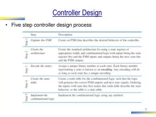
International Journal of Trend in Scientific Research and Development (IJTSRD) ISSN: 2456 International Journal of Trend in Scientific Research and Development (IJTSRD) ISSN: 2456 International Journal of Trend in Scientific Research and Development (IJTSRD) ISSN: 2456-6470 Columns 1 through 10 Inf 17.5500 11.3750 9.5333 8.7750 8.4500 8.3417 8.3571 8.4500 8.5944 Columns 11 through 20 8.7750 8.9818 9.2083 9.4500 9.7036 9.9667 10.2375 10.5147 10.7972 11.0842 Columns 21 through 30 11.3750 11.6690 11.9659 12.2652 12.5667 12.8700 13.1750 13.4815 13.7893 14.0983 Columns 31 through 40 14.4083 14.7194 15.0313 15.3439 15.6574 15.9714 16.2861 16.6014 16.9171 17.2333 Columns 41 through 50 17.5500 17.8671 18.1845 18.5023 18.8205 19.1389 19.4576 19.7766 20.0958 20.4153 Column 51 20.7350 >> Plot (T, K) Fig.1. Advanced D-Partitioning in terms of two variable parameters The D-Partitioning curve K = f (T) border between the region of stability instability D(1) for case of simultaneous variation of the two system parameters. Each point of the D Partitioning curve represents the marginal values of the two simultaneously variable paramete unique advancement and an innovation in the theory of control systems stability demonstration of the system performance in case of variation of the time-constant T isdone at gain set to K = 10. When 0 < T < 0.25 sec and T system is stable. But it becomes unstable in the range < 1.5 sec. It is also obvious that the system performance and stability depends on the interaction between the two simultaneously varying < 8.3417, the system is stable for Higher values of K (K = 12, K = system is stable. But it becomes unstable in the range 0.25 sec < T < 1.5 sec. It is also obvious that the system performance and stability depends on the interaction between the two simultaneously varying parameters. If K < 8.3417, the system any value of the T. Higher values of 14), enlarge the range of T at which the system will fall into instability. III. Design of a Controller for Systems with Simultaneously Variable Parameters The open-loop transfer function of the plant modified and now presented in equation (6) considering the two variable parameters that are the system’s gain K and time-constant suggested that the gain is set to variable [5], [7], [8]. K s GPO Inf 17.5500 11.3750 9.5333 8.7750 8.4500 8.9818 9.2083 9.4500 9.7036 9.9667 at which the system will 11.3750 11.6690 11.9659 12.2652 12.5667 12.8700 13.1750 13.4815 13.7893 14.0983 Design of a Controller for Systems with Simultaneously Variable Parameters function of the plant GP0(s) is modified and now presented in equation (6) the two variable parameters that are the .0313 15.3439 15.6574 15.9714 16.2861 16.6014 16.9171 17.2333 constant T. Initially, it is suggested that the gain is set to K = 10, while T is 17.5500 17.8671 18.1845 18.5023 18.8205 19.1389 19.4576 19.7766 20.0958 20.4153 = = ( ) + 5 . 0 + + K 1 ( )( 1 )( 1 8 . 0 8 ) Ts s s (6) = + + + + + 3 2 4 . 0 3 . 1 ( ) 4 . 0 3 . 1 ( ) 1 Ts T s T s The robust controller consists of a series stage and a forward stage GF0(s). An integrating stage is also included in the controller as seen from 2. The robust controller consists of a series stage GS0(s) (s). An integrating stage GI0(s) is also included in the controller as seen from Figure Fig.2. Robust controller incorporated Robust controller incorporated into the control system system Initially, the plant transfer function standalone block, is involved in a unity feedback system having a closed-loop transfer function presented as: K s GCL + + + 1 )( 5 . 0 1 )( 1 ( Initially, the plant transfer function GP0 (s), as a standalone block, is involved in a unity feedback loop transfer function Partitioning in terms of two = = ( ) + . 0 8 . ) Ts s s K (7) K s ) K (T) defines the = + + + + + + 3 2 border between the region of stability D (0) and instability D(1) for case of simultaneous variation of the two system parameters. Each point of the D- Partitioning curve represents the marginal values of the two simultaneously variable parameters. This is a unique advancement and an innovation in the theory of control systems stability demonstration of the system performance in case of 4 . 0 3 . 1 ( ) 4 . 0 3 . 1 ( ) 1 Ts T T s K Equation (7) is used as a base in the design strategy for constructing the series stage of the robust controller. It has the task to place its two zeros near the desired dominant closed- the condition ζ= 0.707 [9], [10] become the dominant poles of the unity negative feedback system, involving the cascade connection of the series controller stage GS0 Equation (7) is used as a base in the design strategy for constructing the series stage of the robust controller. It has the task to place its two zeros near -loop poles, that satisfy = 0.707 [9], [10]. These zeros will become the dominant poles of the unity negative feedback system, involving the cascade connection of analysis. analysis. The The done at gain set to T > 1.5 sec the S0(s), the integrator GI0(s) @ IJTSRD | Available Online @ www.ijtsrd.com www.ijtsrd.com | Volume – 2 | Issue – 6 | Sep-Oct 2018 Oct 2018 Page: 270
International Journal of Trend in Scientific Research and Development (IJTSRD) ISSN: 2456 International Journal of Trend in Scientific Research and Development (IJTSRD) ISSN: 2456 International Journal of Trend in Scientific Research and Development (IJTSRD) ISSN: 2456-6470 and the plant GP0(s). If initially the gain is set to 10, the optimal value of the time corresponding to the relative damping ratio of the closed-loop system, is determined by the code: >> T= [20:0.01:35]; >> For n=1: length (T) G_array(:,:,n)=tf([10],[0.4*T(n)(1.3*T(n)+0.4) (1.3+T(n)) 11]);end >> [y, z] = damp (G_array); >> [y, z] = damp (G_array); >> Plot (T,z(1,:)) If initially the gain is set to K = ue of the time-constant T, The series robust controller zeros can be placed at the The series robust controller zeros can be placed at the approximated values −0.5 ± transfer function of the series robust controller is: )( 5 . 0 5 . 0 ( ) ( 0 = s GS ± j0.5. Therefore, the corresponding to the relative damping ratio ζ= 0,707 loop system, is determined by the code: transfer function of the series robust controller GS0(s) + + + − j . 0 5 . ) 5 . 0 s j s = 5 . 0 (9) 2 + + 5 . 0 s s (1.3*T(n)+0.4) = 5 . 0 An integrating stage GI0(s) is added to eliminate the steady-state error of the system. It is connected in cascade with the series controller. Then, the transfer function of the compensated open will be as follows: ) ( 0 0 0 ( ) ( ) ( s G s G s G s G P S I OL = (s) is added to eliminate the state error of the system. It is connected in cascade with the series controller. Then, the transfer function of the compensated open-loop control system = = ) (10) 2 + + ( ) 5 . 0 s ) K s s = + + + 5 . 0 1 ( s )( 1 5 . 0 )( 1 1 8 . 0 ) Ts s When GOL(s) is involved in a unity feedback, its closed-loop transfer function is determined as: loop transfer function is determined as: (s) is involved in a unity feedback, its 2 + + ( ) 5 . 0 K s s = ( ) GCL s (11) + + + + 5 . 0 1 ( s )( 1 5 . 0 )( 1 8 . 0 ) Ts s s s 2 + + + ( ) 5 . 0 K s s It is seen from the equation (11) that the closed zeros will attempt to cancel the closed loop poles of the system, being in their area. avoided if a forward controller closed-loop system, as shown in of GF0(s) are designed to cancel the zeros of the closed-loop transfer function equation (12): 5 . 0 ) ( 2 0 + + s s Finally, the transfer function of the total compensated system is derived considering the diagram in = = 0 0 0 ) ( ) ( s G G s G S CL F T It is seen from the equation (11) that the closed-loop zeros will attempt to cancel the closed loop poles of the system, being in their area. This problem can be avoided if a forward controller GF0(s) is added to the loop system, as shown in Figure 2. The poles (s) are designed to cancel the zeros of the loop transfer function GCL(s), as shown in Figure3. Time-constant corresponding to constant corresponding to ζ = 0,707 As seen from Figure 3, the relative damping ratio is ζ= 0.707 when the time-constant is T = 27.06 sec. By substituting the values T = 27.06 sec and equation (7), the transfer function of the closed system becomes: 10 ) ( 2 3 + + s s The assessment of the system proves that the damping ratio becomes ζ= 0.707, when constant is T = 27.06 sec, resulting in system’s desired closed-loop poles −0.466 ± j0.466. These outcomes are determined from the code: >> GCL0=tf([10],[10.824 35.578 28.36 11]) >> damp (GCL0) Eigenvalue Damping Freq. -4.64e-001 + 4.64e-001i 7.07e-001 6.56e -4.64e-001 - 4.64e-001i 7.07e-001 6.56e -2.36e+000 1.00e+000 2.36e+000 2.36e+000 1.00e+000 2.36e+000 relative damping ratio is = 27.06 sec. = 27.06 sec and K = 10 in equation (7), the transfer function of the closed-loop (8) = GCL s = GF s (12) + + 10 . 824 35 . 578 28 . 36 11 s 5 . 0 Finally, the transfer function of the total compensated system is derived considering the diagram in Figure 2. The assessment of the system proves that the relative when the time- = 27.06 sec, resulting in system’s desired j0.466. These outcomes K = (13) 4 3 + + + 2 . 0 . 0 ( 65 ) 2 . 0 Ts T s >> GCL0=tf([10],[10.824 35.578 28.36 11]) 2 2 + + + + + + . 0 ( 65 5 . 0 ) 5 . 0 ( ) 5 . 0 T s s K s s IV. The system is tested for insensitivity to variations of its gain K and its time-constant performance is done before and after applying the performance is done before and after applying the Eigenvalue Damping Freq. (rad/s) Performance of the Compensated System Compensated System The system is tested for insensitivity to variations of constant T. Comparison of its 001 6.56e-001 001 6.56e-001 @ IJTSRD | Available Online @ www.ijtsrd.com www.ijtsrd.com | Volume – 2 | Issue – 6 | Sep-Oct 2018 Oct 2018 Page: 271
International Journal of Trend in Scientific Research and Development (IJTSRD) ISSN: 2456 International Journal of Trend in Scientific Research and Development (IJTSRD) ISSN: 2456 International Journal of Trend in Scientific Research and Development (IJTSRD) ISSN: 2456-6470 robust compensation. Initially at system gain is set to K = 10 and three different values of the time are set successively to T = 0.1 sec, T = 0.8 sec and 2 sec and are substituted in equation (6). The case of T = 0.8 sec, corresponds to the region D(2) and definitely to an unstable control system. The cases of T = 0.1 sec and T = 2 sec, reflect regions D1(0) and D2(0) accordingly and are related to a stable control system. The transient responses of the system before applying the robust compensation are illustrated in Figure 4 and Figure 5 and are achieved by the following codes: >> Gp001= tf ([0 10],[0.04 0.53 1.4 1]) >> Gp02= tf ([0 10],[0.8 3 3.3 1]) >> Gp0fb001= feedback (Gp001, 1) >> Gp0fb02= feedback (Gp02, 1) >> Step (Gp0fb001, Gp0fb02) robust compensation. Initially at system gain is set to erent values of the time-constants The compensated system robustness in the time-domain. Considering the same values of the time-constant, as those used for the assessment of the original system, sec and T = 2 sec at system gain substituting them in equation transfer functions are obtained: transfer functions are obtained: is also examined for domain. Considering the same constant, as those used for the = 0.8 sec and T = (6). assessment of the original system, T = 0.1 sec, T = 0.8 = 2 sec at system gain K = 10 and substituting them in equation (13), the following = 0.8 sec, corresponds to the region D(2) and definitely to an unstable control system. The = 2 sec, reflect regions 10 = ( ) GT s (14) D1(0) and D2(0) accordingly and are related to a 0 = 1 . 0 T 4 3 2 + + 10 + + . 0 04 . 0 53 21 4 . 21 10 s s s s = ( ) GT s (15) 0 The transient responses of the system before applying the robust compensation are illustrated in Figure 4 and = 8 . 0 T 4 3 3 2 + + + + . 0 32 . 1 44 22 1 . 21 10 s s 10 10 s s = ( ) GT s (16) he following codes: 0 = 2 T 4 3 2 + + + + 8 . 0 3 23 23 3 . 21 10 s s s s The step responses, representing the variation of the robust system, shown in Figure 6, are determined by the code: >> GT01=tf([10], [0.04 0.53 21.4 21 10]) >> GT08=tf([10], [0.32 1.44 22.1 21 10]) >> GT20=tf([10], [0.8 3 23.3 21 10]) >> step (GT01, GT08, GT20) The step responses, representing the time-constant variation of the robust system, shown in Figure 6, are >> GT01=tf([10], [0.04 0.53 21.4 21 10]) >> GT08=tf([10], [0.32 1.44 22.1 21 10]) >> GT20=tf([10], [0.8 3 23.3 21 10]) GT20) Fig.4. Step responses of the original control system (T = 0.1sec, T = 2sec at K = 10) 2sec at K = 10) Step responses of the original control system >> Gp008=tf([0 10],[0.32 1.44 2.1 1]) >> Gp0fb008= feedback (Gp001,1) >> step (Gp0fb008) Fig.6. Step responses of the controller (T = 0. 1 sec, T = 0. 8 sec, T = 2 sec at K = 10) Step responses of the system with a robust (T = 0. 1 sec, T = 0. 8 sec, T = 2 sec at K = As seen from Figure 6, due to controller, the control system becomes quite insensitive to variation of the time step responses for T = 0. 1 sec, 2 sec coincide. Since the system is with two variable parameters, now the gain will be changed, applying: 20, while keeping the system’s time 0.8 sec. For comparison of the system’s insensitivity omparison of the system’s insensitivity , due to the applied robust controller, the control system becomes quite insensitive to variation of the time-constant T. The = 0. 1 sec, T = 0. 8 sec and T = Since the system is with two variable parameters, now the gain will be changed, applying: K = 5, K = 10, K = 20, while keeping the system’s time-constant at T = Fig.5. Step responses of the original control system (T = 0.8sec, at K = 10) Step responses of the original control system @ IJTSRD | Available Online @ www.ijtsrd.com www.ijtsrd.com | Volume – 2 | Issue – 6 | Sep-Oct 2018 Oct 2018 Page: 272
International Journal of Trend in Scientific Research and Development (IJTSRD) ISSN: 2456 International Journal of Trend in Scientific Research and Development (IJTSRD) ISSN: 2456 International Journal of Trend in Scientific Research and Development (IJTSRD) ISSN: 2456-6470 to the gain variation before and after applying the robust compensation, initially the suggested values as shown above are substituted in equation transient responses of the original system are illustrated in Figure 7 and 8 and are achieved by the following codes: >> Gp05=tf([0 5],[0.32 1.44 2.1 1]) >> Gp010=tf([0 10],[0.32 1.44 2.1 1]) >> Gp0fb5=feedback (Gp05, 1) >> Gp0fb10=feedback (Gp010, 1) >> Step (Gp0fb5, Gp0fb10) >> Step (Gp0fb5, Gp0fb10) to the gain variation before and after applying the robust compensation, initially the suggested values as shown above are substituted in equation (6). The transient responses of the original system are n Figure 7 and 8 and are achieved by the It is obvious that the cases of correspond to an unstable original control system. Next, the variable gain K = 5, applying to the robust compensated system, keeping the system’s time-constant at values are substituted in equation following outcomes are delivered: following outcomes are delivered: It is obvious that the cases of K = 10 and K = 20, correspond to an unstable original control system. = 5, K = 10, K = 20 will be applying to the robust compensated system, keeping constant at T = 0.8 sec. These values are substituted in equation (13). As a result, the 5 = ( ) GT s (17) 0 = 5 K 4 3 3 2 + + + + . 0 32 . 1 44 12 1 . 11 5 s s s s 10 10 (18) = ( ) GT s 0 = 10 K 4 3 2 + + 20 20 + + + . 0 32 . 1 44 22 1 . 21 10 s s s s (19) = ( ) GT s 0 = 20 K 4 3 2 + + + + . 0 32 . 1 44 42 1 . 41 20 s s s s To compare the system robustness before and after the robust compensation, the step responses for the three different cases, representing the gain variation of the plotted in Figure 9 with the aid of To compare the system robustness before and after the robust compensation, the step responses for the three different cases, representing the gain variation of the robust system, are plotted in Figure the code as shown below: >> GTK5=tf([2.5],[0.16 0.72 6.05 5.5 2.5]) >> GTK10=tf([5],[0.16 0.72 11.05 10.5 5]) >> GTK20=tf([10],[0.16 0.72 21.05 20.5 10]) >> step (GTK5, GTK10, GTK20 tf([2.5],[0.16 0.72 6.05 5.5 2.5]) >> GTK10=tf([5],[0.16 0.72 11.05 10.5 5]) >> GTK20=tf([10],[0.16 0.72 21.05 20.5 10]) GTK20) Fig.7. Step responses of the original control system (K = 5, K = 10 at T = 0.8sec) (K = 5, K = 10 at T = 0.8sec) responses of the original control system >> Gp020=tf([0 20],[0.32 1.44 2.1 1]) >> Gp0fb5=feedback (Gp05, 1) >> Gp0fb10=feedback (Gp010, 1) >> Gp0fb20=feedback (Gp020, 1) >> step (Gp0fb20) Figure9. System’s step respo controller (K = 5, K = 10, K = 20 at T = 0.8 (K = 5, K = 10, K = 20 at T = 0.8 sec) step responses with the robust Again, the system became robust. An additional zero included into the series robust controller stage can further improve the rise time of the system’s step response. An average case is chosen with sec for the assessment of the sys after the application of the robust controller. This case after the application of the robust controller. This case Again, the system became robust. An additional zero included into the series robust controller stage can further improve the rise time of the system’s step An average case is chosen with K = 10 and T = 0.8 sec for the assessment of the system’s performance Fig.8. Step response of the original cont (K = 20 at T = 0.8sec) Step response of the original control system @ IJTSRD | Available Online @ www.ijtsrd.com www.ijtsrd.com | Volume – 2 | Issue – 6 | Sep-Oct 2018 Oct 2018 Page: 273
International Journal of Trend in Scientific Research and Development (IJTSRD) ISSN: 2456 International Journal of Trend in Scientific Research and Development (IJTSRD) ISSN: 2456 International Journal of Trend in Scientific Research and Development (IJTSRD) ISSN: 2456-6470 will differ insignificantly from the other cases of the discussed variable K and T. The performance evaluation is achieved by following code: >> GT10=tf ([10], [0.32 1.44 22.1 21 10]) >> damp (GT10) Eigen value Damping Freq. (rad/s) -4.91e-001 + 4.89e-001i 7.09e-001 6.93e -4.91e-001 - 4.89e-001i 7.09e-001 6.93e -1.76e+000 + 7.88e+000i 2.18e-001 8.07e+000 -1.76e+000 - 7.88e+000i 2.18e-001 8.07e+000 It is seen that the relative damping ratio enforced by the system’s dominant poles is ζ= 0.709, being very close to the objective value of ζ= 0.707. insignificant difference is due to the rounding of the desired system’s poles to −0.5 ± j0.5, during the design of the series robust controller stage. V. Conclusions The D-Partitioning analysis is further advanced for systems with multivariable parameters [8], [9], [10]. The Advanced D-partitioning in case two variable parameters is demonstrating the strong interaction between the variable parameters. Each point of the Partitioning curve represents the marginal values of the two simultaneously variable parameters, being a unique advancement and an innovation in the theory of control systems stability analysis. The design strategy of a robust controller for linear control systems proves that by implementing desired dominant system poles, the controller enforces the required relative damping performance. For systems Type 0, an additional integrating stage ensures a steady-state error equal to zero. The designed robust controller brings the system to a state of insensitivity to the variation of within specific limits of the parameter variations. The experiments with variation of different parameters show only insignificant difference in performance for the different system conditions [10], [11], [12]. For the discussed case, the system becomes quite insensitive to variation of the time constant within the limits 0.1T<T< 10T. The system is quite insensitive to variations of the gain K within the limits 0.5 < 5K. Insignificant step response difference is observed also if the experiment is repeated with observed also if the experiment is repeated with will differ insignificantly from the other cases of the different variation of the gain and different variation different variation of the gain and different variation time-constants values. Since the design of the robust controller is base the desired system performance in terms of relative damping, its contribution and its unique property is that it can operate effectively for any of the system’s parameter variations or simultaneous variation of a number of parameters. This property is by the comparison of the system’s performance before and after the application of the robust controller. demonstrate that the system performance in terms of damping, stability and time response and insensitive in case of any simultaneous variations of the gain and the time-constant within specific limits. The suggested analysis and design for further advancement of control theory in this References 1.Yanev K., Advanced D Analysis of Digital Control Systems with Multivariable Parameters Automatic Control and System Engineering, Delaware, USA, Volume 17(2), pp. December 2017. 2.Yanev K., D-Partitioning Analysis of Digital Control Systems by Applying the Approximation, International Automatic Control (IREACO) pp. 517-523, November 2014. 3.Yanev K, Advanced D-Partitioning Analysis and Comparison with the Kharitonov’s Theorem Assessment, Journal Engineering Science and Technology (JMEST) Germany, Vol. 2 (1), pp. 338 4.Shinners S., Modern Control System Theory Addison-Wesley Publishing Company, pp.369 472, 2004. 5.Driels M., Linear control System Engineering McGraw-Hill International 2006. 6.Golten J., Verwer A., Control System Design and Simulation, McGraw-Hill 278-335, 2001. 7.Bhanot S., Process Control Principles and Applications, Oxford University Press, pp. 170 187, 2010. 8.Yanev K., Anderson G. Multivariable system's parameters interaction and Multivariable system's parameters interaction and . The performance evaluation is achieved by following code: Since the design of the robust controller is based on the desired system performance in terms of relative damping, its contribution and its unique property is that it can operate effectively for any of the system’s parameter variations or simultaneous variation of a number of parameters. This property is demonstrated by the comparison of the system’s performance before and after the application of the robust controller. Tests demonstrate that the system performance in terms of stability and time response remains robust any simultaneous variations 0.32 1.44 22.1 21 10]) Damping Freq. (rad/s) 001 6.93e-001 001 6.93e-001 001 8.07e+000 001 8.07e+000 It is seen that the relative damping ratio enforced by = 0.709, being very = 0.707. This constant within specific The suggested analysis and design is beneficial for further advancement of control theory in this field. insignificant difference is due to the rounding of the j0.5, during the design of the series robust controller stage. Yanev K., Advanced D-Partitioning Stability Analysis of Digital Control Systems with Multivariable Parameters, ICGST, Journal of Automatic Control and System Engineering, Volume 17(2), pp. 9-19, Partitioning analysis is further advanced for systems with multivariable parameters [8], [9], [10]. partitioning in case two variable parameters is demonstrating the strong interaction between the variable parameters. Each point of the D- Partitioning curve represents the marginal values of the two simultaneously variable parameters, being a unique advancement and an innovation in the theory Partitioning Analysis of Digital Control Systems by Applying the Bilinear Tustin International (IREACO), Italy, Vol. 7, (6), 2014. Review Review of of Partitioning Analysis and The design strategy of a robust controller for linear ntrol systems proves that by implementing desired dominant system poles, the controller enforces the required relative damping performance. For systems Type 0, an additional n with the Kharitonov’s Theorem Journal Engineering Science and Technology (JMEST), Vol. 2 (1), pp. 338-344, January 2015. of of Multidisciplinary Multidisciplinary ratio ratio and and system system state error equal to Modern Control System Theory, Wesley Publishing Company, pp.369- The designed robust controller brings the system to a Linear control System Engineering, International Inc., pp.145-222, its parameters within specific limits of the parameter variations. The experiments with variation of different parameters performance for Control System Design and Hill International Inc., pp. the different system conditions [10], [11], [12]. For the discussed case, the system becomes quite insensitive to variation of the time constant within the . The system is quite insensitive Process Control Principles and , Oxford University Press, pp. 170- within the limits 0.5K<K Yanev K., Anderson G. O, Masupe S., . Insignificant step response difference is @ IJTSRD | Available Online @ www.ijtsrd.com www.ijtsrd.com | Volume – 2 | Issue – 6 | Sep-Oct 2018 Oct 2018 Page: 274
International Journal of Trend in Scientific Research and Development (IJTSRD) ISSN: 2456 International Journal of Trend in Scientific Research and Development (IJTSRD) ISSN: 2456 International Journal of Trend in Scientific Research and Development (IJTSRD) ISSN: 2456-6470 robust control design, Journal of International Review of Automatic Control, Vol. 4(2), pp.180 190, March 2011. 9.Behera L., Kar I., Intelligent Systems and Control Principles and Applications, Oxford University Press, pp. 20-83, 2009. 10.Yanev K. M., Design and Analysis of a Robust Accurate Speed Control System by Applying a Digital Compensator, Automatic Control and System Engineering, Delaware, USA, Vol. 16(1), pp. 2016. 11.Megretski A., Multivariable Control systems, Proceedings of Massachusetts Technology, Vol.7 (4), 2010, pp.182 12.Yanev K. M., Digital Optimal Process Control Systems Automatic Control and System Engineering Delaware, USA, Vol. 17(1), pp. Vol. 17(1), pp. 7-18, June 2017. Vol. 16(1), pp. 27-36, April Journal of International Vol. 4(2), pp.180- Megretski A., Multivariable Control systems, Proceedings of Massachusetts (4), 2010, pp.182-189, 2010. Intelligent Systems and Control , Oxford University Institute Institute of of M., Digital Optimal Compensation of Process Control Systems, ICGST, Journal of Automatic Control and System Engineering, Design and Analysis of a Robust Accurate Speed Control System by Applying a ICGST ICGST Journal Journal of of Automatic Control and System Engineering, @ IJTSRD | Available Online @ www.ijtsrd.com www.ijtsrd.com | Volume – 2 | Issue – 6 | Sep-Oct 2018 Oct 2018 Page: 275