Download
1 / 65
650 likes | 800 Views
CONTROLLER DESIGN. ~ Type of compensator ~ Design of compensator in time response ~ Design of compensator in frequency response. Objective. Type of compensator. Basic block diagram. Input. Output. Compensator. Actuator. Plant. +. -.

E N D
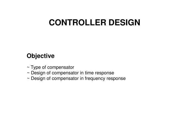
CONTROLLER DESIGN ~ Type of compensator ~ Design of compensator in time response ~ Design of compensator in frequency response Objective
Type of compensator Basic block diagram Input Output Compensator Actuator Plant + - Controller Sensor Actuator Takes low-energy signal to transform and amplify before going to the plant Sensor Takes high-energy signal from plant to transform to low-energy signal for further action
Forward path compensator • Commonly used due to easy implementation + + + -
Feedback path compensator • To avoid time delay and lag + + + -
Feed-forward path compensator • To absorb for disturbance + + + + + -
Inner feedback loop • Also known as cascade control • Used to eliminate any minor disturbance + + + + - -
Velocity feedback • Also known as rate feedback • To overcome the problem of feedback instantaneous change + + + + - -
Selection of compensator (1) Flow • Very noisy, thus need derivative-action • Overall gain less than, integral-action will ensure no steady-state error. (2) Level • Normally is of type 1, thus just required proportional action (3) Temperature • Thermal delay, thus normally required PID-action (4) Pressure • Characteristic can be fast or slow depending on application, thus required PI or P.
PID compensator • Proportional compensator (P) Use to improve steady state error type + R(s) E(s) A(s) Y(s) - B(s) Consider P-compensator transfer function as and where A(s) is the actuator signal. • gives better steady state but poor transient response High • Too high can cause instability.
Example: + - For a unit step input Final value
Integral compensator (I) Use to eliminate error for type 0 Consider the I-compensator and actuating signal of E(s) A(s) + R(s) Y(s) - B(s) • Slow response, can be used with P-compensator to remedy this problem
Example: + - Closed-loop transfer function For a unit step input, the response is
Derivative compensator (D) Derivative compensator (D) Consider the D-compenator as and actuating signal as R(s) + E(s) A(s) Y(s) - B(s) • Quick response • No effect at steady state because no error signal • Useful for controlling type 2 together with a P-controller • Response only to rate of change and no effect to steady state
Example: , , where and Compensator Determine , if damping ratio 0.6 and Error detector Amplifier Servo motor e
New open loop transfer function Give closed loop , , , , For and . C.f. nominal second order dan Hence
Proportional-integral compensator (PI) Use for combination of fast convergence zero steady state error or
Consider a spped control system employing a PI-controller Example: + - Closed-loop transfer function For unit step input
PID Tuning • There are many techniques for tuning PID
Zeigler-Nichols Step Response • Suitable for process control where time lag is significant k 0.63k T a L The above response can be approximated by where k is static gain, T time constant, L time delay and
Based rule-of-thumb, for the controller gains can be appoximated by Controller
Zeigler-Nichols Closed-Loop Method • Using Routh-Hurwitz criteria, we can determined the margainally stable’s gain, and its period • of oscilation, for a controller with a gain of K • With rule-of-thumb of thumb
Design a P, PI and PID controller for a plant with an open loop transfer function as follows Example With a gain of K connected in cascade to the system, its characteristic equaton becomes Forming the Routh array
and its frequency of osccilation which gives T= 1.895 s Thus This gives 1.57 Their step response are
Effect of adding zero and pole Example Consider an open-loop transfer function By introducing a zero and normalizing the response The step response for uncompensated, a=4 and a=8.
The effect of introducing zero • Reduce rise time, peak time • Increases overshoot • As the zero approach the orgin its contribution is more significant • Bandwidth increase • Improve gain margin For a compensator with a pole and normalizing the output The step response for uncompensated, a=4 and a=8.
The effect of introducing pole • Reduce oscillation, and as its more dominant the response becomes sluggish
Design in time response Lag compensator Use for steady state improvement without affecting the transient response Consider a lag compensator transfer function where .
Consider a plant Dc gain without compensator where and zeros and poles position from test point. With compensator As , thus with that the steady state error is reduced.
Lead compensator • For transient response where . Uncompensated Compensated Thus
Example: Use a lead compensator so that the overall system has undamped frequency of 4 rad.s-1 and rate of decay 0.5 s-1, if + - Open loop transfer function
Dominant poles and that give a damping ratio of and Third pole is determined from
s-plane c j3.97 j c -11-10 -1 -0.5 -j c -j3.97
Hence, the dc gain Which give the closed loop transfer function
Location of zero and pole of the system together with the compensator. Satah s s j O -12 -10 -1 -0.5 -j
Using the angle condition on the closed loop poles of where the angle of from i.e. the angle contribution required by Thus the compensator transfer function
Design in frequency response Basic concepts in the design criteria • Increase of phase margin, the overshoot will be reduced • Increase of bandwith, the response will be faster • Increase of low frequency magnitude, the steady state will be reduced
Gain adjustment Use to reduce the overshoot during transeint period by incresing the phase margin dB 0 GM (rad.s-1) Plot LM PM o -180 PM’ Plot Design Procedure (i) With a chosen gain, obtain the Bode plot and the gain crossover frequency, (ii) Determine the required phase margin (iii) Obtain the gain that is required for the new cossover frequency, This gain is the extension of the gain in (i).
Example: Consider a type-1 system. • Determine the uncompensated phase margin. • If a P-compensator is cascaded to the system, determine the requiredgain so that the • phase margin is 30. o + -
By replacing , the frequency response in corner frequency form is Solution: and and and
Pole at origin Real pole Real pole slope and
Real pole Real pole and
>> w1=[1 10 500 10000];LM=[12 -8 -76 -154]; >> w2=[1 50 100 5000 10000];ph=[-90 -166 -193 -269 -269]; >> subplot(2,1,1);semilogx(w1,LM); subplot(2,1,2);semilogx(w2,ph); From the Bode plot, and for uncompensated system