Download
1 / 33
330 likes | 470 Views
Fourier Analysis Without Tears. Somewhere in Cinque Terre, May 2005. 15-463: Computational Photography Alexei Efros, CMU, Fall 2006. x 1. x 1. 1 st principal component. 2 nd principal component. x 0. x 0. Capturing what’s important. Fast vs. slow changes. A nice set of basis.

E N D
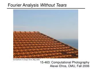
Fourier Analysis Without Tears Somewhere in Cinque Terre, May 2005 15-463: Computational Photography Alexei Efros, CMU, Fall 2006
x1 x1 1st principal component 2nd principal component x0 x0 Capturing what’s important
A nice set of basis Teases away fast vs. slow changes in the image. This change of basis has a special name…
Jean Baptiste Joseph Fourier (1768-1830) • had crazy idea (1807): • Any periodic function can be rewritten as a weighted sum of sines and cosines of different frequencies. • Don’t believe it? • Neither did Lagrange, Laplace, Poisson and other big wigs • Not translated into English until 1878! • But it’s true! • called Fourier Series
A sum of sines • Our building block: • Add enough of them to get any signal f(x) you want! • How many degrees of freedom? • What does each control? • Which one encodes the coarse vs. fine structure of the signal?
Inverse Fourier Transform Fourier Transform F(w) f(x) F(w) f(x) Fourier Transform • We want to understand the frequency w of our signal. So, let’s reparametrize the signal by w instead of x: • For every w from 0 to inf, F(w) holds the amplitude A and phase f of the corresponding sine • How can F hold both? Complex number trick! We can always go back:
Time and Frequency • example : g(t) = sin(2pf t) + (1/3)sin(2p(3f) t)
Time and Frequency • example : g(t) = sin(2pf t) + (1/3)sin(2p(3f) t) = +
Frequency Spectra • example : g(t) = sin(2pf t) + (1/3)sin(2p(3f) t) = +
Frequency Spectra • Usually, frequency is more interesting than the phase
Frequency Spectra = + =
Frequency Spectra = + =
Frequency Spectra = + =
Frequency Spectra = + =
Frequency Spectra = + =
FT: Just a change of basis M * f(x) = F(w) = * . . .
IFT: Just a change of basis M-1 * F(w)= f(x) = * . . .
Finally: Scary Math • …not really scary: • is hiding our old friend: • So it’s just our signal f(x) times sine at frequency w phase can be encoded by sin/cos pair
Extension to 2D in Matlab, check out: imagesc(log(abs(fftshift(fft2(im)))));
Campbell-Robson contrast sensitivity curve We don’t resolve high frequencies too well… … let’s use this to compress images… JPEG!
Lossy Image Compression (JPEG) Block-based Discrete Cosine Transform (DCT)
Using DCT in JPEG • A variant of discrete Fourier transform • Real numbers • Fast implementation • Block size • small block • faster • correlation exists between neighboring pixels • large block • better compression in smooth regions
Using DCT in JPEG • The first coefficient B(0,0) is the DC component, the average intensity • The top-left coeffs represent low frequencies, the bottom right – high frequencies
Image compression using DCT • DCT enables image compression by concentrating most image information in the low frequencies • Loose unimportant image info (high frequencies) by cutting B(u,v) at bottom right • The decoder computes the inverse DCT – IDCT • Quantization Table • 3 5 7 9 11 13 15 17 • 5 7 9 11 13 15 17 19 • 7 9 11 13 15 17 19 21 • 9 11 13 15 17 19 21 23 • 11 13 15 17 19 21 23 25 • 13 15 17 19 21 23 25 27 • 15 17 19 21 23 25 27 29 • 17 19 21 23 25 27 29 31
JPEG compression comparison 89k 12k