Download
1 / 45
450 likes | 647 Views
Shortest Paths. CONTENTS Introduction to Shortest Paths (Section 4.1) Applications of Shortest Paths (Section 4.2) Optimality Conditions (Section 5.2) Generic Label-Correcting Algorithm (Section 5.3) Specific Implementations (Section 5.4) Detecting Negative Cycles (Section 5.5)

E N D
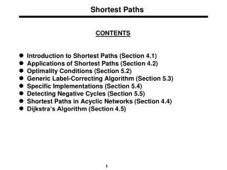
Shortest Paths CONTENTS • Introduction to Shortest Paths (Section 4.1) • Applications of Shortest Paths (Section 4.2) • Optimality Conditions (Section 5.2) • Generic Label-Correcting Algorithm (Section 5.3) • Specific Implementations (Section 5.4) • Detecting Negative Cycles (Section 5.5) • Shortest Paths in Acyclic Networks (Section 4.4) • Dijkstra’s Algorithm (Section 4.5) • Heap Implementations (Section 4.7) • Dial’s Implementation (Section 4.6) • Radix-Heap Implementation (Section 4.8)
20 2 4 10 30 s t 15 40 1 6 35 20 25 3 5 35 Problem Definition Shortest Path Problem: Identify a shortest path from the source node s to the sink node t in a directed network with arc costs (or lengths) given by cij’s. Shortest Path: 1-2-5-6
An Alternative Problem Identify a shortest path from the source node s to every other node in a directed network. 20 2 4 10 30 s 15 40 1 6 35 20 25 3 5 35 • In the process of determining shortest path from node s to node t, we also determine shortest path from node s to every other node in the network, which is specified by a directed out-tree. • We shall henceforth consider this more general problem.
A Linear Programming Problem The shortest path problem can be conceived of as a minimum cost flow problem: Send unit flow from the source node s to every other node in the network. Minimize subject to xij 0 for every arc (i, j) A
Assumptions • All arc costs (or lengths) cij's are integer and C is the largest magnitudes of arc costs. • Rational arc costs can be converted to integer arc costs. • Irrational arc costs (such as, ) cannot be handled. • The network contains a directed path from node s to every other node in the network. • We can add artificial arcs of large cost to satisfy this assumption. • The network does not contain a negative cycle. • In the presence of negative cycles, the optimal solution of the shortest path problem is unbounded. • The network is directed. • To satisfy this assumption, replace each undirected arc (i, j) with cost cij by two directed arc (i, j) and (j, i) with cost cij.
Applications of Shortest Paths • Find a path of minimum length in a network. • Find a path taking minimum time in a network. • In a network G with arc reliabilities given by rij’s, find a path P of maximum reliability (given by (i,j)P rij). • As a subroutine in a multitude of problems: • Minimum cost flow problem • Multi-commodity flow problems • Network design problems
Determining Optimal Rental Policy • Beverly owns a vacation rental which is available for rent for three months, say May 1 to July 31. • She has received many bids, each having the following form: the day the rental starts (a rental day starts at 3 p.m.), the day the rental ends (checkout time is noon), and the money (in dollars) the renter will pay for this duration. • Beverly wants to determine the bids she should accept so as to maximize her total revenue.
1 3 5 2 4 6 Determining Optimal Rental Policy (contd.) • Define a node for each rental day from May 1 to July 31. • Define an arc (i, j) for each bid - node i corresponding to the starting day of the bid, node j corresponds to the ending day of the bid, and cij is the bid amount. • Define an arc (i, i+1) for each node i with zero cost (denoting that the house is vacant). • Show that there is a one-to-one correspondence between the rental policy and the directed paths from the first node to the last node.
Additional Applications • Paragraph Problem: A paragraph is a sequence of consecutive words which are partitioned into lines. The paragraph problem consists of decomposing the words into lines so as to maximize its total attractiveness. • Optimal Tree Cutting Policy: You own a plot large enough for a single tree. At various times, you cut down the tree to obtain some wood to sell. You want to determine how to maximize your revenue from selling the wood during the next 100 years. • Equipment Replacement Problem: A job shop must periodically replace its capital equipment due to machine wear. Obtain a replacement plan that minimizes the total cost of buying, selling, and operating the machine over a planning horizon of n years, assuming that the job shop must have at least one unit of machine in service at all times.
System of Difference Constraints • We are given a following set of m difference constraints in nvariables and we wish to know whether it possesses a feasible solution: x(jk) – x(ik) b(k) for each k = 1, 2, … , m. • Example: x(3) – x(2) 2; x(2) – x(1) -11 x(1) – x(3) 8; x(3) – x(4) 5; x(4) – x(1) -10
System of Difference Constraints (contd.) • Example: x(3) – x(2) 2; x(3) – x(4) 5; x(4) – x(1) -10 x(1) – x(3) 8; x(2) – x(1) -11 • The system of difference constraints has a feasible solution if and only if the following network has no negative cycle.
Distance Labels • Most shortest path algorithms maintain a distance label d(i) for each node i. • The distance label d(i) represent the cost (or, length) of some directed path from the source node s to node i. 10 30 20 2 4 10 30 15 40 1 6 0 90 35 20 25 3 5 35 45 70 • Distance labels are upper bounds on shortest path distances.
Optimality Conditions Theorem 1: If distance labels d(i)'s represent shortest path distances, then they must satisfy the following conditions: d(j) d(i) + cij for every arc (i,j) A. d(i) i cij d(s) s j d(j) = cij + d(i) - d(j) Theorem 1 (Alternate): If distance labels d(i)'s represent shortest path distances, then they must satisfy the following conditions: 0 for every arc (i, j) A.
Optimality Conditions (contd.) Theorem 1: If distance labels d(i)'s satisfy 0 for every arc (i, j) A, then they represent shortest path distances. Proof. Let P be any directed path from node s to node k. Since d(s) = 0 and 0 for each arc (i, j), we get d(k) implying that d(k) is a lower bound on the length of every path from node s to node j. Since d(k) is the length of some path from node s to node k, it must be the shortest path distance.
20 2 4 10 30 15 40 1 6 35 20 25 3 5 35 Generic Label-Correcting Algorithm algorithm label-correcting; begin d(s) : = 0 and pred(s) : = 0; d(j) : = for each j N - {s}; while some arc (i, j) satisfies d(j) > d(i) + cijdo begin d(j) = d(i) + cij; pred(j) : = i; end; end; Numerical Example:
Running Time of the Generic Algorithm 1. Time needed to perform an iteration: O(m) 2. Number of iterations: O(n2C) • Each distance label d(i) is bounded from above by nC • Each distance label d(i) is bounded from below by -nC • Each iteration decreases some distance label by at least one unit 3. Total running time: O(n2mC) {pseudo-polynomial time)
j i l s k q p An O(nm) Implementation 1. Examine each arc one by one, check its optimality condition, and update distance labels. 2. Repeat the above process (passes over the arc list) until in the entire pass no distance label is updated. Theorem. After kth pass, the algorithm will determine shortest path distances to all those nodes whose shortest path contains k or lesser number of arcs. Proof: By induction on k. Nodes with shortest paths containing k arcs or less
An Improved Generic Algorithm How to identify an arc violating its optimality condition quickly? Property 1. If an arc (i, j) satisfies its optimality condition at some step, then it continues to satisfy its optimality condition until either d(j) increases or d(i) decreases. Property 2. In the generic algorithm, distance labels only decrease but never increase. IDEA: Maintain a list, LIST, of nodes whose distance labels have decreased and examine arcs emanating from such nodes. Stop when LIST is empty.
An Improved Generic Algorithm (contd.) algorithm label-correcting; begin d(s) : = 0 and pred(s) : = 0; d(j) : = for each j N - {s}; LIST : = {s}; while LIST 0 do begin remove an element i from LIST; for each (i, j) A(i) do if d(j) > d(i) + cijthen begin d(j) = d(i) + cij; pred(j) : = i; if j LIST then add j to LIST; end; end; end;
Properties of Generic Algorithm Property 1: At termination, predecessor indices give the Tree of Shortest Paths. Property 2: Whenever d(i) decreases, node i is added to LIST, and O(|A(i)|) arcs are examined. Property 3: -nC d(i) nC. Hence any d(i) decreases O(nC) times. Property 4: The generic label-correcting algorithm runs in O(iNnC|A(i)|) time = O(nmC) time.
Features of Generic Algorithm • Quite flexible since nodes in LIST can be examined in any order. • By examining nodes in certain specific order we can obtain an O(nm) algorithm - one of the best algorithms from the worst-case complexity point of view. • We can examine nodes in another order to obtain the best algorithm from empirical point of view. • An O(m) implementation for acyclic networks. • An O(n2) implementation for networks with nonnegative arc lengths.
Queue Implementation • Examines nodes in the FIFO (first-in-first-out) order. • Always removes nodes from the front of LIST for examination. • Always adds new nodes to the rear of the LIST. • It can be shown that any node is examined at most n times.
Dequeue Implementation • Very efficient in practice, but only pseudo-polynomial in the worst-case. • Examines nodes in a dequeue fashion [dequeue is a doubly ended queue] . • Always removes nodes from the front of LIST examination. • Adds a new node to the rear of LIST if the node has never been in the LIST before, otherwise to the front of LIST. • Why the dequeue implementation runs very well in practice?
Negative Cycle Detection Property: If the network contains a negative cycle, then the optimality condition can never be satisfied. Proof: (i) Let W be a negative cost directed cycle. Hence (ii) Optimality conditions imply that 0 for every arc (i, j) in W. (iii) Both (i) and (ii) cannot be true simultaneously. Property: If the network contains a negative cycle, then the label-correcting algorithm will never terminate.
20 4 2 10 10 10 1 5 3 5 Numerical Example of Negative Cycle Detection • Apply FIFO label correcting algorithm and count the number of times a node is examined. • If a node is examined more than n times, then network contains a negative cycle. • Predecessor indices can be used to identify the negative cycle. -50
Shortest Paths in Acyclic Networks • A network is called acyclic if it does not contain any directed cycle. • We can solve shortest path problem in acyclic networks in O(m) time. • For an acyclic graph, nodes can be topologically ordered, that is, can be ordered such that for each arc (i, j) A, i < j.
15 50 4 7 3 20 5 30 1 10 10 5 6 2 5 15 50 Algorithm algorithm acylic-shortest-path; begin order nodes in the topological order; for each node i in the topological order do for each arc (i, j) in A(i) do d(j) : = min{d(j), d(i) + cij}; end;
k j s Proof of Correctness Proof: By induction on the number of nodes examined. Induction Hypothesis: When the algorithm has examined nodes 1, 2, 3, ... , k-1, then it has correctly determined shortest path distance to node k. Consider a shortest path from node s to node k. Since the network is acyclic, j < k.
Dijkstra’s Algorithm • Dijkstra's algorithm is one of the most efficient shortest path algorithm. Dijkstra's algorithm is a label-setting algorithm. • Always examines a node with the minimum distance label and no node is examined more than once. • Nodes have distance labels which are either permanent or temporary. • Permanent labels are shortest path distances and do not change. • Temporary labels are estimates of shortest path distances and may change. • In each iteration, the algorithm makes a temporary distance label permanent.
20 2 4 10 30 15 10 5 1 6 5 25 3 5 30 Numerical Example of Dijkstra’s Algorithm
Dijkstra’s Algorithm algorithm Dijkstra; begin d(s) : = 0 and pred(s) : = 0; d(j) : = for each j N - {s}; LIST : = {s}; while LIST f do begin let d(i) : = min{d(j) : j LIST}; (Node Selection) remove node i from LIST; for each (i, j) A(i) do (Distance Update) if d(j) > d(i) + cijthen begin d(j) : = d(i) + cij; pred(j) : = i; if j LIST then add j to LIST; end; end; end;
Analysis of Dijkstra’s Algorithm Two Major Steps: • Node Selection: Identifying a node i with the minimum distance label. • Distance Update: Scanning arcs emanating from node i Running Time Analysis: (i) Time for node selection (selecting minimum distance label nodes) = O(n2). (ii) Time for Distance Updates = O(iA |A(i)|) = O(m). Total Time = O(m + n2) = O(n2)
S i j s t k Proof of Correctness S : Set of permanently labeled nodes : Set of temporarily labeled nodes Induction Hypothesis: • Distance label d(j) of each node j in S is the shortest path distance. • Distance label d(j) of each node j in is the shortest path distance among those paths containing only the nodes in S as internal nodes.
Heap Implementations of Dijkstra’s Algorithm (contd.) • Dijkstra’s algorithm can be implemented in a variety of ways using different heap data structures. • A HEAP is a data structure which maintains a set H (heap) of objects where each object i has an associated key[i] and allows the following (heap) operations: • insert(i, H) : Adding an object i to the heap H • find-min(i, H) : Find and return an object i of minimum key • delete-min(i, H) : Delete an object of minimum key • decrease-key(value, i, H) : Reduce the key of object i from its current value to value, which must be smaller than the key it is replacing
Heap Implementations of Dijkstra’s Algorithm (contd.) • While implementing Dijkstra’s algorithm, we store LIST (nodes with temporary distance label) as a heap and d(i) as the key of node i.
Dial’s Implementation • An implementation of Dijkstra's algorithm which is very efficient in practice. • Uses the property that distance labels made permanent by Dijkstra's algorithm are non-decreasing. • Uses (1+nC) buckets, numbered 0, 1, 2, ... , nC. • Bucket k holds all nodes whose distance labels equal k as a doubly-linked list.
9 2 4 1 4 6 5 2 1 6 8 8 3 5 3 Dial’s Implementation (contd.)
Dial’s Implementation (contd.) • Node Selection Operation: Scan the buckets in the increasing order until a nonempty bucket is found. In the next iteration, we start where we left off earlier. • Distance Update Operation: Same as earlier except that the contents of the buckets must be updated after each distance update. If d(j) changes 6 to 3 then node j is moved from bucket 6 to bucket 3. • Time for node selections : O(nC) • Time for distance updates : O(m) • Total time : O(m + nC)
Radix Heap Implementation • Due to Ahuja, Mehlhorn, Orlin and Tarjan. • Improved version of Dial's implementation with running time of O(m + n log(nC)). • Under the similarity assumption (that is, C = O(nk) for some constant k), the running time is O(m + n log n). • Uses buckets of progressively larger widths which change dynamically.
5 2 4 15 2 13 1 6 20 4 0 3 5 9 i 2 3 4 5 6 d( i) 13 0 15 20 bucket k 0 1 2 3 4 5 6 7 range (k) [0] [1] [2,3] [4,7] [8,15] [16,31] [32,63] [64,127] content k {3} f f f {2,4} {5} f f Radix Heap Implementation 5 Iteration 1. Make node 1 permanent and update distance labels 13 15 2 4 15 2 13 0 1 6 20 4 0 3 5 20 0 9
Radix Heap Implementation (contd.) 5 Iteration 2. Make node 3 permanent and update distance label of node 5 13 15 2 4 15 2 13 0 1 6 0 20 4 0 3 5 9 0 9
Radix Heap Implementation (contd.) 5 Redistribute the range of bucket 4, and move nodes to the appropriate buckets. 13 15 2 4 15 2 13 0 1 6 0 20 4 0 3 5 9 0 9
Radix Heap Implementation (contd.) 5 Iteration 3. Make node 5 permanent and update distance labels of node 6 to 14. 13 15 2 4 15 2 13 0 1 6 14 20 4 0 3 5 9 0 9
Radix Heap Implementation (contd.) Iteration 3. Redistribute the range of bucket 3 and move nodes to the right buckets. 5 13 15 2 4 15 2 13 0 1 6 14 20 4 0 3 5 9 0 9
Running Time Analysis • Number of buckets K = 1 + log(nC) = O(log(nC)) • Number of iterations = n • Time for identifying lowest-index nonempty bucket O(K) per iteration and O(nK) overall • Time for redistribution of bucket ranges O(K) per redistribution and O(nK) overall • Time for redistribution of nodes O(K) per node and O(nK) overall • Time for distance updates O(m) for arc scannings and O(nK) for node distributions • Total Time = O(m + nK) = O(m + n log(nC))