Download
1 / 38
390 likes | 572 Views
2.2 Shortest Paths. Def : directed graph or digraph : of nodes, of arcs, functions associating to each , a tail and a head . A digraph is called simple if it has no loops or parallel (same directions) arcs. write for , forward arc, reverse arc in a path

E N D
2.2 Shortest Paths • Def: • directed graph or digraph: of nodes, of arcs, functions associating to each , a tail and a head . • A digraph is called simple if it has no loops or parallel (same directions) arcs. • write for , • forward arc, reverse arc in a path • A path in which every arc is forward is a directed path or dipath • A dicircuit is a dipath that is also a circuit • Shortest path problem Input: A digraph , a node , and a real cost vector ( : ) Objective: To find, for each , a (simple)dipath from to of least cost (if one exists). • Assume that there exist dipaths from to every node and is simple. (We may add arcs from to with large costs to ensure the existence of dipaths)
Overview of results • Directed graphs: • longest path problem difficult • If is acyclic, easy (e.g., PERT network) • Shortest path problem: • If does not contain negative-cost dicircuit, easy. • If contains a negative-cost dicircuit, there exist algorithms which can detect it but they cannot find a directed simple path. (all combinatorial algorithm tries to find min cost dipath, not necessarily a simpledipath) • Finding shortest simple path is difficult (when negative-cost dicircuit exists) • Acyclic graph, nonnegative arc costs: easy
Undirected graphs: • longest path problem difficult • If is acyclic, easy • Shortest path problem: • If has nonnegative edge costs: easy • replace each edge by two directed arcs with opposite direction and apply the algorithm for directed case. • modify the algorithm for directed case. • If negative edge cost allowed: • Note that doubling an edge with directed arcs having negative cost and using algorithm for directed case does not work. • If contains a negative-cost circuit, difficult to find a shortest simple path. • If does not contain a negative-cost circuit, can be solved as a join problem (later)
Ideas: Let denote the length of a shortest dipath from to for each . Then it must satisfy for all (2.12) (Otherwise, and the path from to gives a shorter path.) We call a feasible potential if it satisfies (2.12) and (Note that we can subtract from each and (2.12) still satisfied) • Proposition 2.9: Let be a feasible potential and let be a dipath from to . Then . Pf) Suppose is where and Then .
Proposition 2.9 shows that a feasible potential gives a lower bound for the shortest path costs. Suppose we have a feasible potential. Then, if we can find paths to each which satisfies (2.12) at equality for the edges on each path to , they give paths having as path lengths. So we have proofs that they are actually the shortest paths to . • Moreover, the shortest paths do not use many arcs in . We can assume that all the shortest paths use only one arc having head for each node . (Subpaths of a shortest path are shortest paths) Hence, the subgraph of which consists of arcs in the shortest dipaths forms a spanning tree (only arcs and connected) (arborescence). This subgraph can be identified by storing the information of the immediate predecessor of node ().
Algorithm strategy (1) Maintain and update a spanning tree (arborescence) which actually gives paths to each node (may not be shortest). The values represent the path length of some path to (It may not be the path length to in the current tree). (2) Try to find feasible potential by selecting arc which violates (2.12) , then update (decrease) the potential of to . If potential is updated, update the predecessor of node as , if necessary. (3) If we have found a feasible potential and spanning tree , it is optimal shortest spanning tree and is shortest path length.
Ford’s Algorithm • We call an arc violating (2.12) incorrect. To correct means to set and to set • Initializing the algorithm: Set , , , for • Ford’s algorithm: Initialize , ; While is not a feasible potential Find an incorrect arc and correct it.
a (Example) 2 3 r d 1 1 b
Remark • For arc , if , we disregard arc (arc does not grow tree) • Good implementation prevent this situation • When correcting arc , two cases occur • : update (), update the unique predecessor of in . • : no change in , update • holds in the tree at termination, but it may not be true before termination. (consider after 4th iteration) • holds throughout. (It held with equality when and were assigned their current values and after that can only decrease. If decreases, changes. )
a (Abnormal case) 1 2 r b 1 -3 d
Application involving negative-cost dicircuit: currency exchange rate If we can find a sequence of currency transactions such that , we can make money. • Form a digraph whose nodes are currencies, with an arc of cost for each pair . Then a sequence of transactions is money making iff associated dipath has cost . • Existence of money-making sequence can be checked by checking the existence of a negative-cost dicircuit in .
Shortest Path and LP • Consider an IP formulation to find a shortest path (not the paths from to every other nodes). Define if if otherwise IP formulation is minimize subject to , for all (i.e. inflow – outflow = net flow at node , flow conservation) , and integer for all
Consider the LP relaxation and its dual: (P) minimize subject to , for all , for all (D) maximize subject to for all • The coefficient matrix of constraints in (P) has special structure; each column has exactly one 1 and one –1 (except nonnegativity constraints). Such matrix is totally unimodular (details later). For totally unimodular matrix, if the rhs is integer valued, any basic feasible solution to LP is integral. Hence, there exists an integer optimal solution if an optimal solution exists and, from strong duality, optimal values of (P) and (D) are equal.
From the constraints of (D), we can see that is a feasible potential iff it is a feasible dual solution (with ). For any feasible dual solution (feasible potential), , gives a lower bound on the optimal shortest path length from to , , as was shown. • Using CS conditions, we can see that the dual constraints hold at equality for the edges on the optimal path (for fixed ) in an optimal solution.
Abnormal case (existence of negative cost dicircuit) If the network has a negative-cost dicircuit, the LP is unbounded, hence dual is infeasible. 1 1 1(M) 2(M) s r -5(M) Let flow of M on the dicircuit • We may increase the flow over the negative-cost dicircuit indefinitely, hence the LP is unbounded. Although we may impose the restriction that on each arc, then the optimal solution is not a simple path.
Validity of Ford’s Algorithm • Prop 2.10: If has no negative-cost dicircuit, then at any stage of the Ford’s algorithm we have : (i) If , then it is the cost of a simpledipath from to . (ii) If , then defines a simpledipath from to of cost at most . pf) (i) Let be the value of after iterations. If , it is a cost of some dipath from to (The dipath may not be the same as the dipath to in the current arborescence). To prove that it is simple, suppose that it includes a closed dipath and derive contradiction. Then there exists and such that , The cost of the resulting dipath is . But was lowered at iteration , hence the dipath has negative cost, contradiction.
(ii) Similar to (i). If does not define a simple dipath, there exists and for . For an arc in the selected subgraph (arborescence), we always have . ( note that , never increase ) Hence total cost of the closed dipath is . In the most recent predecessor assignment in the closed dipath, the potential of the head node strictly decreases. Suppose is such node and new node potential is . Then . So a negative-cost closed dipath exists, contradiction. Next, consider a dipath where and for . The cost of dipath is
Thm 2.11: If has no negative-cost dicircuit, then Ford’s algorithm terminates after a finite number of iterations. At termination, for each , defines a least-cost dipath from to of cost . pf) only finitely many simple dipaths in , hence possible values for finite by Prop 2.10. One of decreases strictly in each iteration and never increases, hence finitely terminates. At termination, (pointers) defines a simple dipath from to of cost at most , but is lower bound on shortest path to if is feasible potential.
Thm 2.12: has a feasible potential iff it has no negative-cost dicircuit. pf) If has a feasible potential, then no negative-cost dicircuit ( since for all ) Suppose has no negative-cost dicircuit. Add a node to and connect to for with cost 0. has no negative-cost dicircuit since no dicircuit goes through . Now apply Ford’s algorithm to . has a dipath from to all other nodes, hence produces feasible potential and it is also feasible potential for . Note that the theorem holds without the assumption of the existence of dipaths to all .
Running time of Ford’s Algorithm: Each step decreases some by at least one. Let max Prop 2.13: If is integer-valued, and has no negative-cost dicircuit, then Ford’s algorithm terminates after at most arc-correction steps.
Feasible Potentials and Linear Programming • Thm 2.14: Let be a digraph, and . If there exists a least-cost dipath from to for every , then Min{ : a dipath from to } = max{ : a feasible potential } • Recall from earlier: (P) minimize (2.14) subject to , for all , for all (D) maximize (2.13) subject to for all
If (2.14) has a finite optimal solution, it has an integer optimal solution, which is the simple path (when no negative-cost dicircuit exists). (2.14) has an integer optimal solution for all choices of if finite optimal solution exists, which implies that the polyhedron is integral (every extreme point is integer vector). • The constraint matrix in (2.14) has special structure; each column has exactly one 1 and one –1 (except nonnegativity constraints). Adding the rows of the matrix , we get 0 vector, which implies the rows are linearly dependent (rank is ). • Prop 2.15: Let be a connected digraph and be its incidence matrix ( is the column vector for arc in the constraint matrix) . A set is a column basis of iff is the arc-set of a spanning tree of (not considering the directions of the arcs). ( has nodes, arcs. is matrix. Spanning tree has arcs.)
So the rank of is . To solve the problem by the simplex method, we need nonsingular basis . Two approaches: • Drop one of the constraints and solve the full row rank problem • Add an artificial variable to any one constraint (objective coefficient is 0). It makes full row rank (the artificial variable always remains in the basis and has value 0 in any b.f.s). • b.f.s. and dual vector satisfies for all for all ( From for current basis ) This vector gives the path length to each node in the current tree (If is arborescence). Note that if we add artificial variable for node (root), then we have in any bfs (from )
A bfs for (2.14) does not necessarily correspond to an arborescence (each node has one predecessor except node ) . It may be just a spanning tree. However, the simplex iteration can be modified so that we always have arborescence once we started the algorithm with an arborescence. • Each step of the simplex method may correspond to multiple Ford’s step; (1) Change of arborescence (2) update the node potentials so that it gives the actual path length in the arborescence.
Suppose we solve shortest path problem by LP (with simplex method) and have a feasible arborescence (bfs); • entering nonbasic arc selection: choose with , i.e. . ( from since we solve min problem ) • leaving basic variable: select the entering arc to in the current arborescence as leaving basic variable. • Update flow (value) so that we have value 1 for each arc on the path. • Note that we may solve the shortest path problem by LP. But, in an optimal basis (arborescence), we have shortest path, for all . ( If you use the above modified simplex method) ( We have feasible potential and the paths in the arborescence for all gives actual path with length for all .)
The identification of the basis of the LP as a spanning tree (not necessarily arborescence) is used in the primal minimum cost flow algorithm for the minimum cost network flow problem. (Chapter 4)
Refinements of Ford’s Algorithm • Number of steps depends on the sequence we consider the arcs. • Let be the sequence of arcs considered (arcs may be repeated). Let denote the dipath where . After the first time Ford’s algorithm considers , we will have . After the first subsequent time Ford’s algorithm considers , we will have . Continuing, once the arcs in the path are considered in the order they appear in the path, we have . We say that is imbeddedin if its arcs occur (in the right order, but not necessarily consecutively) as a subsequence of .
Prop 2.16: If Ford’s algorithm uses the sequence , then for every and for every path from to embedded in S, we have . • If contains the sequence for all optimal path to , we have for all path to and for all . Also the pointer defines a simple dipath to with cost at most . Hence the algorithm stops.
The Ford-Bellman Algorithm • Use the sequence such that each edge is considered once in a pass. Let be an ordering of . Then every simple dipath in is embedded in the sequences . If is not a feasible potential after passes, there exists a negative-cost dicircuit. Ford-Bellman Algorithm Initialize ; Set ; While and is not a feasible potential replace by ; For If is incorrect Correct .
Refinements: Store the arcs having tail in a list . Scan means For If is incorrect Correct ; Replace the last 3 statements of the algorithm by For Scan ;
Note that if has not decreased since the last time was scanned, then need not be scanned Keep a list of nodes to be scanned Initially Add node to when is decreased and . Choose the next node to be scanned from (and delete it from ) Stop the algorithm when is empty. Keep as both a list (or queue) and a characteristic vector.
Acyclic Digraphs • Topological sortof nodes in : Ordering of of so that implies . • If we can order in the sequence so that precedes if , then every dipath in is imbedded in . Hence Ford’s algorithm solves the problem in one pass ( ). • has a topological sort if and only if is acyclic. (pf) If has a topological sort, then clearly it has no dicircuit. Conversely, if is acyclic, then there exists a node such that for no . Let the node be and eliminate it from . Then is also acyclic and repeat the procedure.
Nonnegative Costs • When we choose the node to be scanned next, select the node for which is minimum. Then we have • Prop 2.19: For each , let be the value of when is chosen to be scanned. If is scanned before , then . pf) Suppose and let be the earliest node scanned for which this is true. When was scanned, we had . So was lowered to a value after was scanned and before was scanned. So for some node , was set to . By choice of , and since , we have . Contradiction.
After all nodes are scanned, we have for all . Suppose not. Then was lowered after was scanned, say while node was scanned. Then was set to since was scanned later than and . Contradiction. Dijkstra’s Algorithm Initialize ; Set ; While Choose with minimum; Delete from ; Scan .
We have for since . So only need to test if for . • Running time: + time to find {} Hence total time is • Notation:: time needed to solve a nonnegative cost shortest path problem on a digraph with nodes and arcs • If we happen to know the feasible potential , then may transform so that we can use Di’s algorithm. Any dipath satisfies , hence shortest path does not change.
Unit Costs and Breadth-First Search • Prop 2.21: If each , then in Di’s algorithm the final value of is the first finite value assigned to it. Moreover, if is assigned its first finite before is, then . pf) True for . If , the first finite value is for some , where is the final value of . Moreover, any node scanned later than has by Prop 2.19, so will not be further decreased. Similarly, any node assigned its first finite after will have for some . • Hence, when picking , we choose the first element in queue of unscanned nodes having finite. => breadth-first search. can be found in constant time, hence running time is Need when we consider an algorithm for maximum flow problem.
Other Interpretation of Ford-Bellman Alg. • Handout: Combinatorial Optimization: Networks and Matroids, E. Lawler • Bellman’s equations: , • Initial values , Iteration • Interpretation the length of a shortest path from the origin to , subject to the condition that the path contains no more than arcs.
M Shortest Paths without Repeated Nodes • Handout: Combinatorial Optimization: Networks and Matroids, E. Lawler • Enumerate simple paths in nondecreasing order with respect to the weights. • Not efficient, but useful when we want to find a shortest path satisfying, or not satisfying certain conditions additionally imposed. • Suppose we have shortest paths . Let be the set of all paths. We divide the set into , where . Each includes paths with the condition that (a) they include the arcs in a certain specified path from node to another node , and (b) certain arcs from node are excluded. Then we can find a shortest path in by finding a shortest path from node to after deleting nodes in the path from to , and deleting the arcs excluded from node .