Download
1 / 56
560 likes | 596 Views
Understand the concept of conservative weights in graph theory and learn how Dijkstra's Algorithm computes shortest paths. Explore the principles and proofs involved in solving the shortest paths problem efficiently.

E N D
Shortest Paths Problem • Instance: A digraph G, weights c: E(G) → R and two vertices s, t V(G). • Task: Find a s-t-path of minimum weight.
Conservative weights • Definition 5.1. Let G be a (directed or undirected) graph with weights c: E(G) → R . c is called conservative if there is no circuit of negative total weight.
Bellman’s principle of optimality Proposition 5.2. Let G be a digraph with conservative weights c: E(G) → R, and let s and w be two vertices. If e=(v, w) is the final edge of some shortest path P from s to w, then P[s,v](i.e. P without the edge e) is a shortest path from s to v.
Proof • SupposeQ is a shorter s-v-path thanP[s,v]. • Thenc(Q) + c(e) < c(P). • Ifw Q, thenQ + eis a shorter s-w-path thanP. • Contradiction wQ.
Доказательство (wQ) • LetQ be a shorter s-v-path thanP[s,v] and c(Q) + c(e) < c(P). • c(Q[s,w]) = c(Q) + c(e) – c(Q[v,w]+e) < < c(P) – c(Q[v,w]+e) • SinceQ[v,w]+eisa circuit, thenc(Q[s,w])< c(P) – c(Q[v,w]+e)≤ c(P). • Contradiction. Q w Q v P s
Remark • The same result holds for undirected graphs with nonnegative weights and also for acyclic digraphs with arbitrary weights. It yields the following recursion formulas. • dist(s,s) = 0. • dist(s,w) = min{dist(s,v) + c((v,w)): (v,w) E(G)} for wV(G)/s.
Shortest paths from One Source • Proposition 5.2 is also the reason why most algorithms compute the shortest paths from s to all vertices. • If one computes a shortest s-t-path, one has already computed a shortest s-v-path for each vertex v on P. • Since we cannot know in advance which vertices belong to P, it is natural to compute shortest s-v-paths for all v.
Dijkstra’s Algorithm Input: A digraph G, weights c: E(G) → R+and a vertex s V(G). Output: Shortest paths from s to all v V(G) and their lengths. • Set l(s) 0. Set l(v) for all v V(G)\{s}. Set R . • Find a vertex v V(G)\R such that l(v) = min w V(G)\{R}l(w). • Set R R ∪{v}. • For all w V(G)\R such that (v,w) E(G)do: If l(w) > l(v) + c((v,w))then set l(w) l(v) + c((v,w))and p(w) v. 5) If R ≠ V(G) then go to 2.
Step 1 x= 1 y= 1 3 3 s=0 t= 1 2 1 2 w= z=
Step 2 … Step 5 x=1 1 y= R = {s} 1 3 3 s=0 t= 1 2 1 2 w= z=2
Step 2 … Step 5 x=1 1 y=2 R = {s, x} 1 3 4 s=0 t= 1 2 1 2 z=2 w=5
Step 2 … Step 5 x=1 1 y=2 R = {s, x, y} 1 3 4 s=0 t=5 1 2 1 2 z=2 w=3
Step 2 … Step 5 x=1 1 y=2 1 3 4 s=0 t=4 1 2 1 2 z=2 w=3 R = {s, x, y, z, w, t}
Dijkstra’s Algorithm (2) Theorem 5.3. (Dijkstra [1959]) Dijkstra’s Algorithm works correctly. Its running time is O(n2), where n=|V(G)|.
Sketch of Proof We prove that the following statements hold each time that step 2 is executed in the algorithm. a) For all v R and all w V(G)\R: l(v) ≤l(w). b) For all v R: l(v) is the length of a shortest s-v-path in G. If l(v) < , there exists an s-v-path of length l(v) whose final edge is (p(v),v) and whose vertices all belong to R. c) For all w V(G)\R: l(w) is the length of a shortest s-w-path in G[R∪{w}]. If w ≠ s andl(w) ≠ then p(w) R and l(w) = l(p(w)) + c((p(w), w)).
Dijkstra’s Algorithm Input: A digraph G, weights c: E(G) → R+and a vertex s V(G). Output: Shortest paths from s to all v V(G) and their lengths. • Set l(s) 0. Set l(v) for all v V(G)\{s}. Set R . • Find a vertex v V(G)\R such that l(v) = min w V(G)\{R}l(w). • Set R R ∪{v}. • For all w V(G)\R such that (v,w) E(G)do: If l(w) > l(v) + c((v,w))then set l(w) l(v) + c((v,w))and p(w) v. 5) If R ≠ V(G) then go to 2.
a) For all v R and all w V(G)\R: l(v) ≤l(w). • Letv be the vertex chosen in step 2. • For any x R andy V(G)\R: l(x) ≤l(v) ≤l(y). • a) continues to hold after 3,and so after 4.
b) For all v R: l(v) is the length of a shortest s-v-path in G. If l(v) < , there exists an s-v-path of length l(v) whose final edge is (p(v),v) and whose vertices all belong to R. • Sincec)was true before (3), it suffices to show that no s-v-path inGcontaining some vertex of V(G)\Ris shorter than l(v). • Suppose there is ans-v-pathP inG containingw V(G)\R, which is shorter thanl(v). • Letwbe the first vertex outside Rwhen traversing P from s to v. • Sincec)was true before (3) l(w) ≤ с(P[s,w]) • Since the edge weights are nonnegative, с(P[s,w]) ≤ с(P) < l(v). • l(w) < l(v), contradicting the choice of v in step 2.
c) For all w V(G)\R: l(w) is the length of a shortest s-w-path in G[R∪{w}]. If w ≠ s andl(w) ≠ then p(w) R and l(w) = l(p(w)) + c((p(w), w)). • Suppose after (3)and(4) there is an s-w-pathP inG[R⋃w]which is shorter than l(w)for some w V(G)\R. • Pmust containv, the only vertex added to R, for otherwise с) would have been violated before 3 and 4. • Let x be the neighbour of w in P, i.e. (x,w) P. • x R & a) l(x) ≤l(v). • Step 4 l(w) ≤l(x) + c((x,w)) ≤ l(v) + c((x,w)). • b) l(v) is the length of a shortest s-v-path. • P containss-v-path as well as the edge (x,w) l(w) ≤l(x) + c((x,w)) ≤ c(P). • Contradiction with our assumption.
Moore-Bellman-Ford Algorithm Input: A digraph G, weights c: E(G) → R+and a vertex s V(G). Output: Shortest paths from s to all v V(G) and their lengths. • Set l(s) 0 andl(v) for all v V(G)\{s}. • For i 1 to n – 1do: For each edge (v,w) E(G)do Ifl(w) > l(v) + c((v,w))then l(w) l(v) + c((v,w))and p(w) v.
Step 1 x= 1 y= 1 3 3 s=0 t= 2 1 -3 2 1 2 w= z=
Step 2 x=1 1 y= 1 3 3 s=0 t= 2 1 -3 2 1 2 w= z=2 p(x)=s, p(z)=s
Step 2 x=1 1 y=-1 1 3 3 s=0 t= 2 1 -3 2 1 2 w=4 z=2 p(x)=s, p(z)=s, p(y)=z, p(w)=z
Step 2 x=0 1 y=-1 1 3 3 s=0 t=2 2 1 -3 2 1 2 z=2 w=0 p(x)=y, p(z)=s, p(y)=z, p(w)=y
Step 2 x=0 1 y=-1 1 3 3 s=0 t=1 2 1 -3 2 1 2 z=2 w=0 p(x)=y, p(z)=s, p(y)=z, p(w)=y, p(t)=w
Moore-Bellman-Ford Algorithm (2) Theorem 5.4. (Moore [1959], Bellman [1958], Ford [1956]) The Moore-Bellman-Ford Algorithm works correctly. Its running time isO(nm).
Sketch of Proof At any stage of the algorithm let R {v V(G): l(v) < } and F {(x,y) E(G): x= p(y) }. We claim a) l(y) ≥ l(x) + c((x,y)) for all (x,y) F ; b) If F contains a circuit C, then C has negative total weight; c) If c is conservative, then (R, F) is an arborescence rooted at s.
a) l(y) ≥ l(x) + c((x,y)) for all (x,y) F • F {(x,y) E(G): x= p(y)} • Consider the last iteration when l(y) has changed. • Observe thatl(y) =l(x) + c((x,y)) whenp(y)is set tox. • l(x)is never increased.
b) If F contains a circuit C, then C has negative total weight; • Suppose at some stage a circuit C in F was creating by setting p(y) x (we add edge (x,y) to F) • Then before the insertion we had l(y) >l(x) + c((x,y)). • a) l(w) ≥l(v) + c((v,w)) for all(v,w)E(С)/{(x,y)}. • Summing these inequalities, we see that the total weight of C is negative. w v x y
Moore-Bellman-Ford Algorithm Input: A digraph G, weights c: E(G) → R+and a vertex s V(G). Output: Shortest paths from s to all v V(G) and their lengths. • Set l(s) 0 andl(v) for all v V(G)\{s}. • For i 1 to n – 1do: For each edge (v,w) E(G)do Ifl(w) > l(v) + c((v,w))then l(w) l(v) + c((v,w))and p(w) v.
c) If c is conservative, then (R, F) is an arborescence rooted at s. • b) F is acyclic. • Moreover, x R\{s}implies p(x) R (R,F) is an arborescence rooted ats. • Therefore l(x) is at least the length of thes-x-pathin(R,F) for anyx Rat any stage of algorithm. • We claim that after k iterations of the algorithm l(x) is at most the length of a shortest s-x-pathwith at most k edges.
After k iterations of the algorithm l(x) is at most the length of a shortest s-x-pathwith at most k edges. • LetP be a shortests-x-path with at mostk edges and let (w,x) be the last edge ofP. • ThenP[s,w] must be a shortests-w-path with at mostk–1edges. • By the induction hypothesis we have l(w) ≤ c(P[s,w]) afterk –1iterations. • But in the k iteration edge (w,x) is also examined, after which l(x) ≤l(w) + c((w,x)) ≤ c(P). • Since no path has more than n – 1edges, the above claim implies the correctness of the algorithm.
Moore-Bellman-Ford Algorithm (2) Theorem 5.4. The Moore-Bellman-Ford Algorithm works correctly. Its running time isO(nm).
Feasible potential • Definition 5.5. Let G be a digraph with weights c: E(G) → R, and let : V(G) → R. Then for any (x,y) E(G) we define the reduced cost of (x,y) with respect to by c((x,y)) c((x,y)) + (x) – (y). If c(e) ≥ 0 for all e E(G), is called a feasible potential.
Feasible potential (2) Theorem 5.6. Let G be a digraph with weights c: E(G) → R. There exists a feasible potential of (G,c) if and only if c is conservative.
Proof • Ifis a feasible potential, we have for each circuitC: • c is conservative. • On the other hand, if c is conservative,we add a new vertex sand edges (s,v) of zero cost for all v V(G). • We run the Moore-Bellman-Ford Algorithm on this instance and obtain numbers l(v)for allv V(G). • Since l(v)is the length of a shortests-v-path for allv V(G). • l(w) ≤l(v) + c((v,w))for all(v,w) E(G). • Hence l(v) is a feasible potential.
Feasible potential (3) Corollary 5.7. Given a digraph G with weights c: E(G) → Rwe can find in O(nm) time either a feasible potential or a negative circuit.
Proof • We add a new vertex s and edges (s,v) of zero cost for all v V(G). We run the Moore-Bellman-Ford Algorithm on this instance: Regardless of whether c is conservative or not. • We obtain numbers l(v) for all v V(G). If l is a feasible potential, G does not contain a negative circuit. • Otherwise let (v,w) be any edge with l(w) >l(v) + c((v,w)). • We claim that the sequence w, v, p(v), p(p(v)), … contains a circuit.
l(w) >l(v) + c((v,w)) The sequence w, v, p(v), p(p(v)), … contains a circuit. • Observe that l(v) must have been changed in the final iteration of (2). Hence l(p(v)) has been changed during the last two iterations, l(p(p(v))) has been changed during the last three iterations, and so on. • Since l(s) never changes, the first n places of the sequence w, v, p(v), p(p(v)), … do not contain s, so a vertex must appear twice in the sequence. • Thus we have found a circuit C in F {(x,y) E(G): x= p(y)}∪{(v,w)}. • By (a) and (b) of the Theorem 5.4, C has negative total weight.
All Pairs Shortest Paths Problem • Instance: A digraph G, weights c: E(G) → R. • Task: Find number lstand vertices pst for all s, t V(G) withs≠ t, such that lst isthe length of a shortest s-t-path, and (pst , t) is the final edge of such a path (if it exists).
All Pairs Shortest Paths Problem(2) Theorem 5.8. The All Pairs Shortest Paths Problem can be solved in O(n3) time (where n = |V(G)|).
Proof • Let (G,c) be an instance. • First we compute a feasible potential , which is possible in O(nm) time by Corollary 5.7. • Then for each s V(G) we do a single-source shortest path computation from s using the reduced costs c instead of c. • For any vertex t the resulting s-t-path is also a shortest path with respect to c, because the length of any s-t-path changes by (s) – (t), a constant. • Since the reduced costs are nonnegative, we can use Dijkstra’s Algorithm each time. • So the total running time is O(mn + nn2) = O(n3).
Floyd-Warshall Algorithm Input: A digraph G with V(G) = {1,...,n} and conservativeweights c: E(G) → R. Output: Matrices (lij)1≤i,j≤nand (pij)1≤i,j≤nwhere lij is the length of a shortest path from i to j and (pij ,j) is the final edge of such a path (if it exists). • Set lij c((i, j)) for all (i, j) E(G). Set lij for all (i, j) (V(G)× V(G))\ E(G) with i≠j. Set lii 0 for all i. Set pik i for all i, k V(G). • For j 1 to n do: For j 1 to n do:If i≠j then: For k 1 to n do:If k≠j then: If lik>lij + ljk then set liklij + ljk and pikpjk
Step2 For j 1 to n do: For i 1 to n do:If i≠j then: For k 1 to n do:If k≠j then: If lik>lij + ljkthen set liklij + ljk and pikpjk k pjk j i
Floyd-Warshall Algorithm (2) Theorem 4.9.(Floyd [1962], Warshall [1962]) TheFloyd-Warshall Algorithmworks correctly. Its running time isO(n3).
Claim • After the algorithm has run through the outer loop for j=1, 2, …, j0, the variablelikcontainsthe length of a shortest i-k-path with intermediate vertices v {1, 2, …, j0}and (pik,k) is the final edge of such a path. • This statement will be shown by induction for j0=0 ,…, n. For j0 = 0 it is true by (step 1), and for j0 = n itimplies the correctness of the algorithm.
j0→ j0+ 1 For anyi andk, during processing the outer loop forj = j0+ 1:lik is replaced bylij + ljk , if this value is smaller. {1, 2, …, j0} k Q P j=j0+1 i Letlikgot new value. It remains to show that the corresponding i-(j0+ 1)-path P and (j0+ 1)-k-path Q have no inner vertex in common.
j0→ j0+ 1 Letlikgot new value. It remains to show that the corresponding i-(j0+ 1)-path P and (j0+ 1)-k-path Q have no inner vertex in common. {1, 2, …, j0} k Q P j=j0+1 Suppose that there is a inner vertex belonging to both P and Q. By shortcutting the maximal closed walk in P + Q we get an i-k-path R with intermediate vertices v {1, 2, …, j0} only. R isno longer than i
Metric closure • Definition 4.10.