Download
1 / 98
990 likes | 997 Views
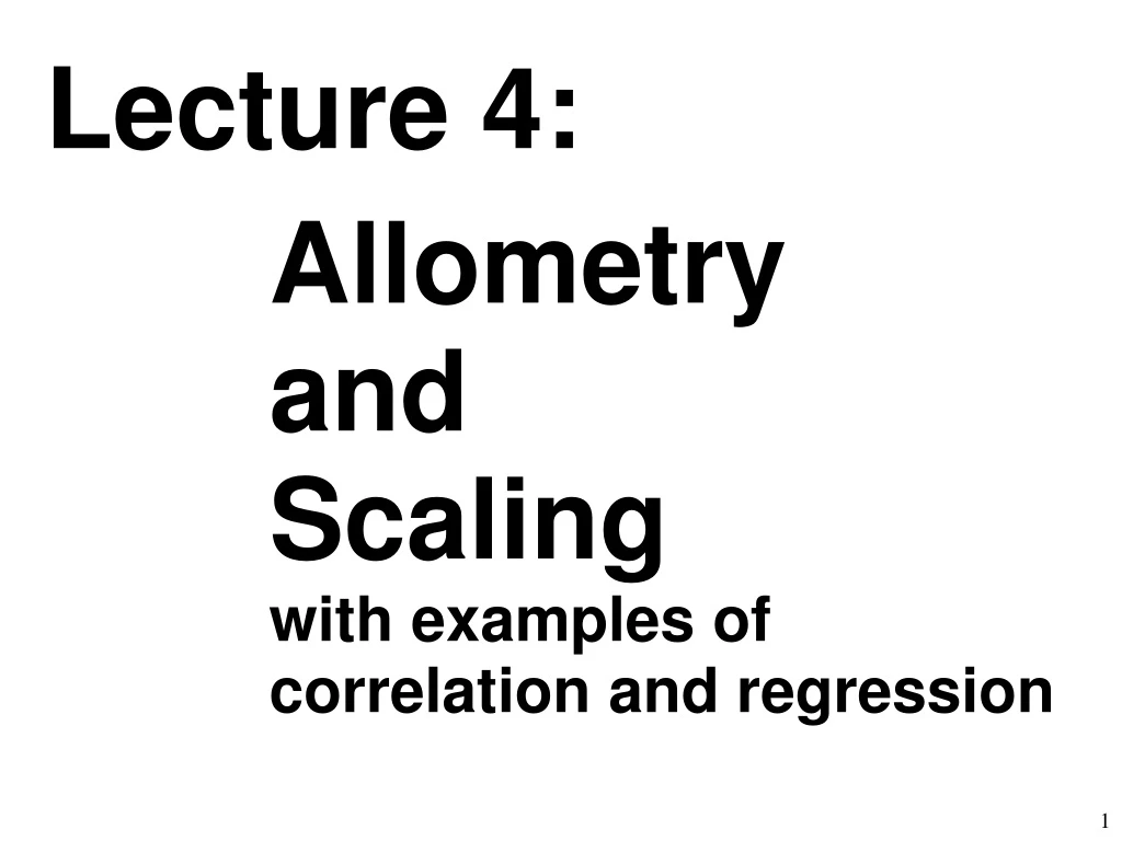
Lecture 4: Allometry and Scaling with examples of correlation and regression. Allometry = "different measure" = the study of how and why properties of organisms change in regular ways in relation to body size. Scaling = essentially a synonymous term in biology, but used more in engineering.

E N D
Lecture 4: • AllometryandScalingwith examples of correlation and regression
Allometry = "different measure" = the study of how and why properties of organisms change in regular ways in relation to body size. Scaling = essentially a synonymous term in biology, but used more in engineering. Can be studied at three levels: 1. ontogenetic (intraspecific) = growth relationships during development, between two traits or between one trait and the whole organism: a. longitudinal = follow individuals b. cross-sectional = mixed-age sample
Allometric Growth in Human Beings: Juveniles are not Scale Models of Adults (http://en.wikipedia.org/wiki/Scale_model)
Zebrafish: again, large changes in shape are occurring ... Randall, D., W. Burggren, and K. French. 2002. Eckert animal physiology: mechanisms and adaptations. 5th ed. W. H. Freeman and Co., New York.
Allometric growth is differential rates of growth of two or more traits. It is often well described by the equation:Y = bXa where Y is one trait (e.g., metabolic rate), b is a constant, a is the "allometric" or "scaling" coefficient, and X is the other trait (often a measure of body size, e.g., mass or length).
Y = bXa This equation describes a logarithmic relationship. It can be made linear by taking the logs of the values measured for each trait, or by plotting on log-log graph paper. If we take logs, then the equation becomes: log Y = log b + a log X This equation describes a straight linewith a being the slope.
"Reptiles" (not a good term, phylogenetically speaking) are a good model for studies of ontogenetic allometry because: 1. they have little or no parental care, so newly hatched or born offspring must fend for themselves, forage, escape from predators, etc.; 2. huge size rangefrom juvenile to adult; 3. no metamorphosis to complicate the picture.
An Example of Studying Ontogenetic Allometry: Amphibolurus (Ctenophorus) nuchalisfrom central Australia Australian National Bird Recent Hatchling Adult Male Adult Female
Fowler’s Gap: a Research Station and Working Sheep Ranch run by the University of New South Wales
Fowler’s Gap: a Research Station and Working Sheep Ranch run by the University of New South Wales
Area around Fowler’s Gap: Lizards often Bask on Fence Posts, or use them for Territorial Outposts
Convergent Evolution with North American Dipsosaurus dorsalis (desert iguana) Amphibolurus (Ctenophorus) nuchalis
Exponent (slope of line) is < 1, so liver exhibits negative ontogenetic allometry
log base 10 version 95% Confidence Interval on slope is 0.747 - 1.063
Logarithmic axes. Note that the log transform also: 1. shrinks large values, expands small 2. homogenizes variances
Exponent (slope of line) is > 1, so thigh muscle exhibits positive ontogenetic allometry
95% Confidence Interval on slope is 1.104 - 1.212 Juveniles are not just scale models of adults!
Relationship is non-linear even on log-log scale. Again, juveniles are not just miniature adults!
Non-linear ontogenetic allometries (on log-log scale) of physiological traits also occur in garter snakes and water snakes, and in many amphibians around metamorphosis. The common garter snake, Thamnophis sirtalis
Rattlesnake tail-shaker muscle contraction frequency varies across ontogeny in a highly non-linear fashion. http://www.sloanmonster.com/images/snake2.jpg https://c2.staticflickr.com/2/1331/794381822_d015c02a30.jpg Moon, B. R., and A. Tullis. 2006. The ontogeny of contractile performance and metabolic capacity in a high-frequency muscle. Physiological and Biochemical Zoology 79:20-30.
Muscle contractile frequency is related to muscle aerobic capacity across ontogenetic development. Moon, B. R., and A. Tullis. 2006. The ontogeny of contractile performance and metabolic capacity in a high-frequency muscle. Physiological and Biochemical Zoology 79:20-30.
An Altricial Mammal, the house mouse Randall, D., W. Burggren, and K. French. 2002. Eckert animal physiology: mechanisms and adaptations. 5th ed. W. H. Freeman and Co., New York.
Some Differences between Hatchling and Adult Amphibolurus (Ctenophorus) nuchalis: Ratio 1 g 50 g 50/1 Liver, % body mass 3.4 2.3 0.69 Heart, % body mass 0.27 0.40 1.51 Thigh, % body mass 1.31 2.44 1.86 Hindlimb span/SVL 1.52 1.25 0.82 Hematocrit (%) 6.0 20.7 3.44 How might these differences affect organismal performance? Stopped here 13 Jan. 2015
Amphibolurus (Ctenophorus) nuchalis slope = 0.16 Maximal Sprinting Speed (km/h) Body Mass (g) Started here 15 Jan. 2015 Closed circles are juveniles and adult males. Closed triangles are females. Line is for all of these animals.Open circles are gravid females. Open squares are long-term captives. Star is adult male captured missing lower portion of right leg below knee.
Amphibolurus (Ctenophorus) nuchalis Closed circles and solid regression line are January animals. Open circles and dashed line are March animals. Open triangles represent 4 gravid females. Star is adult male captured missing lower portion of right leg below knee. slope = 0.65 Garland, T., Jr., and P. L. Else. 1987. Seasonal, sexual, and individual variation in endurance and activity metabolism in lizards. Am. J. Physiol. 252 (Regulatory Integrative Comp. Physiol. 21):R439-R449.
Take-home Messages for the Lizard Ontogenetic Allometry Example: • Juveniles are not "scale models" of adults;they are not just miniature adults. • They differ in both shape and physiological functions. • The scaling of locomotor performance (speed, stamina) could not have been predicted simply from the scaling of the lower-level traits presented (e.g., muscle mass, hematocrit). • However, development of mechanistic models may allow us to get there in the future …
Additional levels at which allometry can be studied: 2. static = size relationships of traits among individuals of the same age (typically adults) 3. evolutionary (interspecific) = size relationships among species This is a perennial favorite of comparative and ecological physiologists! It pervades the fields. Many books have been written.
Books on Allometry (mainly interspecific): Brown, J. H., and G. B. West, eds. 2000. Scaling in biology. Oxford Univ. Press, New York. Calder, W. A. 1984. Size, function and life history. Harvard Univ. Press, Cambridge. Peters, R. H. 1983. The ecological implications of body size. Cambridge Univ. Press, Cambridge. Reiss, M. J. 1989. The allometry of growth and reproduction. Cambridge Univ. Press, Cambridge. Schmidt-Nielsen, K. 1984. Scaling: why is animal size so important? Cambridge Univ. Press, Cambridge.(You do not need to remember all of these, but note that you have a reading from the last one.)
Allometry also Occurs at Behavioral Levels 49 Species of Mammals Carnivora Eat Herbivores log10 Home Range Area (km2) ungulates Slope = 1.26 (from a phylogenetic analysis ) Eat Plants log10 Body Mass (kg) Garland, T., Jr., A. W. Dickerman, C. M. Janis, and J. A. Jones. 1993. Phylogenetic analysis of covariance by computer simulation. Systematic Biology 42:265-292. See also: Dial, K. P., E. Greene, and D. J. Irschick. 2008. Allometry of behavior. Trends in Ecology & Evolution 23:394-401.
Allometry also Occurs at an Ecological Level solid line = slope of -0.75 Damuth, J. 2007. A macroevolutionary explanation for energy equivalence in the scaling of body size and population density. American Naturalist 169:621-631.
Allometry: Predictions from First Principles; A Tool to Understand Organismal Design and Adaptation
Scaling Relationships Based on First Principles For geometrically similar objects (scale models): Relationships with Length Circumference Length1(for a circle, circumference 2 * π * radius1) Cross-sectional Area Length2(for a circle, area π * radius2) Surface Area Length2 Volume Length3(for a sphere, volume 4/3 π * radius3) Mass Length3(assuming that density remains constant)
Consider a cube ... Length 1 2 3 C-S Area 1 4 9 Circum- 4 8 12 ference Surface 6 24 54 Area Volume 1 8 27 S.A./Vol. 6 3 2
Relationships with Mass Volume is proportional to Mass1.00 Length is proportional to Mass0.33 Surface Area is proportional to Mass0.67 Predictions for geometrically similar animals: Blood Volume is proportional to Mass1.00 Mass of Organ is proportional to Body Mass1.00 Limb Length is proportional to Body Mass0.33 Skin, Gill or Lung Surface Area Mass0.67
Allometric Expectations Based on First Principles for Geometrically Similar Objects (scale models) serve as Null Models for Comparison with Real Organisms. • Deviations from "isometry"may indicate how evolution has modified organisms from geometric similarity in order to maintain (more or less) functional abilities across a range of body sizes. • (Only may indicate because this presumes that evolutionary changes in size because of random genetic drift, in the absence of selection, would occur along lines of geometric similarity …)
Example: Mammalian Skeletal Mass As body mass becomes larger, would need bone strength to keep up. Strength cross-sectional area, so would need bone cross-sectional area M1.00 to support the load. Mass of skeleton would be M1.00 X M0.33 = M1.33needed c-s area X length Empirical result: skeletal mass M1.08+0.04 So, large mammals should not be able to do what small ones do (unless all are "over-designed"). In fact, large mammals have more upright postures, less dynamic & less risky locomotor behavior (elephants don’t jump).
Example: Metabolic Rate Amount of (metabolically active) tissue should dictate the rate at which an animal produces heat (or consumes oxygen). Oxygen consumption at rest or during maximum exertion should be M1.00 However, respiratory exchange surface area should be M0.67 "Houston, we have a problem …"
Expected Surface Area, e.g., lung, gill M0.67 Expected Maximal Metabolic Rate M1 Expected Resting Metabolic Rate M1 Max. O2 consumption is typically10-fold higher than Resting log10 scale,Body Mass on X axis
What gives? Metabolic rate typically scales with an exponent less than unity, often ~ 0.7-0.8 (many exceptions).
Randall, D., W. Burggren, and K. French. 2002. Eckert animal physiology: mechanisms and adaptations. 5th ed. W. H. Freeman and Co., New York.
What gives? Metabolic rate typically scales with an exponent less than unity, often ~ 0.7-0.8 (many exceptions). Gas exchange surface area often scales with an exponent greater than 0.67. But, the slopes do not always match. Example: mammalian maximal oxygen consumption (measured on motorized treadmill) scales as M0.872
Scaling of Maximal Metabolic Rate (Exercise) in Mammals slope = 0.87 Weibel, E. R., L. D. Bacigalupe, B. Schmitt, and H. Hoppeler. 2004. Allometric scaling of maximal metabolic rate in mammals: muscle aerobic capacity as determinant factor. Respiratory Physiology & Neurobiology 140:115-132.
What gives? Metabolic rate typically scales with an exponent less than unity, often ~ 0.7-0.8 (many exceptions). Gas exchange surface area often scales with an exponent greater than 0.67. But, the slopes do not always match. Example: mammalian maximal oxygen consumption (measured on motorized treadmill) scales as M0.872 whereas pulmonary diffusing capacity (measured morphometrically) scales as M1.084 So, large-bodied species have excess capacity.
Why the apparent excess capacityin large mammals? Presumably, other things vary allometrically,such as: • blood volume • blood oxygen carrying capacity (hemoglobin, hematocrit) • oxygen unloading characteristics (shape of oxygen dissociation curve, e.g., P50) • capillary densities • capillary transit times • mitochondrial volume densities
Resting and Maximal Metabolic Rates do not always Scale in Parallel. Example: Amphibolurus (Ctenophorus) nuchalis ontogenetic allometry VO2max scales as M0.948 95% C.I. on slope = 0.885 - 1.011 S.M.R. scales as M0.830 95% C.I. on slope = 0.783 - 0.877