Solving ODE

1. Solving ODE Professor Walter W. Olson Department of Mechanical, Industrial and Manufacturing Engineering University of Toledo

2. Outline of Today’s Lecture • Review • SIMULINK • Two common mathematical problems is controls • Numerical Methods • Newton Raphson • Homogeneous Solution • Euler Method • RungeKutta

3. Simulink

4. SIMULINK

5. SIMULINK

6. SIMULINK

7. Two Mathematical Problems Frequently Encountered in Controls • Find the roots of an equation • Methods • Trial and Error (bracketing methods add a bit of science to this) • Graphics • Closed form solutions (e.g.: quadratic formula) • Newton Raphson • Find the solution at a given time for given conditions • Various differential and difference equations analytic solutions (sometimes reformulated as find the roots problem) • Numerical Methods • Newton Cotes Methods (trapezoidal rule, Simpson’s rule. etc. for integration) • Euler’s Method • RungaKutta/Butcher Methods • Many other techniques (Adams-Bashforth, Adams-Milne, Hermite–Obreschkoff, Fehlberg, Conjugate Gradient Methods, etc.)

8. Numerical Methods • Solutions can be approximated using numerical methods • Why Numerical Methods? • Analytical methods may not exist to solve for the exact roots or the exact solution • Use of computers • Flexibility of making changes

9. Numerical Methods • Numerical methods follow the procedure • Step1: Initialize: Select some initial value • Step2: Estimate using (guess, some analytical technique) a new value at increment “i” • Step 3: Is the system converging? If not, use something else. We usually know a priori whether a method will converge or not form mathematics. Therefore, this step is often omitted. • Step 4: Is the change from the previous value to current value smaller than our acceptable error? • If not, make the current value the previous value and return to step 2. • If so, stop and accept the new value as the solution.

10. Newton Raphson Method for finding roots • Probably the most common numerical technique • simple • efficient • flexible • It can be shown from a truncated Taylor’s Series that • Provided that the slope at the test points is consistent, we can iterate to a solution within our error tolerance f(t) f(ti) ti+1 ti Problems occur if the slope reverses sign such as in an oscillation or becomes very flat t

11. Example • Find the roots of To within 0.01 of the value of s • There appears to be a crossing between -2 and 0, but where?

12. ODE for Linear Control Theory • In Linear Control Theory, the equations that are encountered are almost always of the form with constant coefficients subject to initial conditions. Most problems are 2nd order. The electric motor example: Subject to {Va(0), ia(0)=0 and q(0) = 0}

13. Solution Methods • To solve We can use • Reduction in order • Undetermined coefficients • Variation of parameters • Laplace Transforms • Superposition of particular integrals • Cauchy-Euler equation • Numerical methods

14. Reduction of Order • The object is to reduce the order of the equation by substitutions until it can be solved • Example: A hanging cable with a weight of w per unit length under tension T: T y q H s x W

15. Homogenous Case When we form the characteristic equation and solve for its roots We have three possible outcomes for the roots that we must consider: 1) Real Distinct Roots : for p distinct real roots, the solution term is of the form 2) Repeated Real Roots: Assume roots r and r+1 are repeated, that is, Then the term in the solution corresponding to the repeated root is and if there were v repeated roots of the same value, the term would be 3) Complex Conjugate Roots: Assume that roots, The corresponding term of the solution is Therefore the complete solution accounting for all possible roots is

16. Homogenous Example A weight of 15 Kgf is supported (x = 0, at rest,) by a spring with a spring rate of 50 N/m. At t = 0, the weight is extended by 20 centimeters and released. Model and solve.

17. Euler Method Prediction yi • Our goal is to solve equations of the form • The theory for the Euler method is the same as that of the Newton Raphson Method: • Rather than now solve for an axis crossing, we predict where the next value of the curve will be and then • Make successive estimates of yi+1 yi+1 } Error xi xi+1 } step h

18. Example

19. Example • Try a smaller time step,say, h = 0.01seconds

20. RungeKutta/Butcher Method • Has its origins in a 2 variable Taylor Series Expansion • The function is called the increment function • RK4 is a four factor expansion of the incrementing function • For RK4: • Butcher’s method uses 5 factors is more accurate than RK4 at a given time step

21. Example

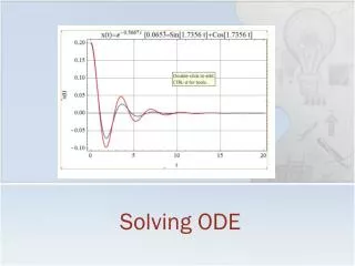
22. Example The result of the RK4 at h = 0.1 is essentially the same as the analytic solution:

23. Summary • Models for Control Systems are either differential equation or difference equations • The problems we commonly see will be • Finding the roots of the equation • Finding the trajectory or path of the equation over time • While we have a number of analytical techniques to find exact results, we cannot address all of the equations encountered • Numerical methods for finding roots and for trajectories are most commonly used • Newton Raphson for finding roots • Methods such as the RungeKutta 4 are used for trajectories Next Class: Analyzing stability