Download
1 / 35
350 likes | 520 Views
Solving Methods for ODE. 전자 20021267 도영욱 물리 20052317 홍용준. Introduction. Program 9.1. Introduction. Use Runge-Kutta Method to solve a second-order ODE. M, B and K is mass, damping constant and spring constant, respectively. Contents. Problem & Code Analysis Methods

E N D
Solving Methods for ODE 전자 20021267 도영욱 물리 20052317 홍용준
Introduction Program 9.1
Introduction • Use Runge-Kutta Method to solve a second-order ODE • M, B and K is mass, damping constant and spring constant, respectively
Contents • Problem & Code • Analysis • Methods • Iterations (Modified Euler Method) • Time Interval
Solution (1) • Modify equation • M = 0.5, B = 10, k = 100
Solution (2) • Solve by using characteristic equation (apply initial values)
Code for(count = 0; count < CYCLE; count++) { step++; time = TIME_INTERVAL * step; y = exp(-10 * time) * (cos(10 * time) + sin(10 * time)); z = (-20) * exp(-10 * time) * sin(10 * time); }
Forward Euler Method(1) • Equations
Forward Euler Method(2) for(count = 0; count < CYCLE; count++) { step++; time = TIME_INTERVAL * step; oldy = y; oldz = z; y = oldy + TIME_INTERVAL * oldz; z = oldz - TIME_INTERVAL * (20 * oldz + 200 * oldy); }
Modified Euler Method for(count = 0; count < CYCLE; count++) { step++; time = TIME_INTERVAL * step; oldy2 = y; oldz2 = z; for(iteration = 0; iteration < iter[mode]; iteration++) { oldy = y; oldz = z; y = oldy2 + TIME_INTERVAL / 2 * (oldz + oldz2); z = oldz2 - TIME_INTERVAL / 2 * (20 * (oldz + oldz2) + 200 * (oldy + oldy2)); } }
Runge-Kutta Method km = k / m; bm = b / m; for(count = 0; count < CYCLE; count++) { step++; time = TIME_INTERVAL * step; k1 = TIME_INTERVAL * z; l1 = -TIME_INTERVAL * (bm * z + km * y); k2 = TIME_INTERVAL * (z + l1); l2 = -TIME_INTERVAL * (bm * (z + l1) + km * (y + k1)); y = y + (k1 + k2) / 2; z = z + (l1 + l2) / 2; }
Analysis in graphs • 1 second • Methods (Δt = 0.01) • Forward Euler Method • Modified Euler Method (5 iterations) • Runge-Kutta Method • Iterations (Modified Euler Method, Δt = 0.01) • 1, 2, 5, 10 • Time Interval (Runge-Kutta Method) • Δt = 0.05 • Δt = 0.01 • Δt = 0.005
Introduction Program 9.3
Solution • Modify equation
RK4[y0_, z0_, time_, Dt_] := Module[{t, y, z, f0, g0}, t[n_] := n Dt; y[0] = y0; z[0] = z0; f0 := f[t[n-1], y[n-1], z[n-1]]; g0 := g[t[n-1], y[n-1], z[n-1]]; k1 := Dt f0; l1 := Dt g0; k2 := Dt f[t[n-1] + Dt/2, y[n-1] + k1/2, z[n-1] + l1/2]; l2 := Dt g[t[n-1] + Dt/2, y[n-1] + k1/2, z[n-1] + l1/2]; k3 := Dt f[t[n-1] + Dt/2, y[n-1] + k2/2, z[n-1] + l2/2]; l3 := Dt g[t[n-1] + Dt/2, y[n-1] + k2/2, z[n-1] + l2/2]; k4 := Dt f[t[n-1] + Dt, y[n-1] + k3, z[n-1] + l3]; l4 := Dt g[t[n-1] + Dt, y[n-1] + k3, z[n-1] + l3]; y[n_] := (y[n] = y[n-1] + (k1 + 2 k2 + 2 k3 + k4)/6); z[n_] := (z[n] = z[n-1] + (l1 + 2 l2 + 2 l3 + l4)/6); Table[{y[n], z[n]}, {n, 0, time/ Dt}]; Ysol = Table[{t[n], y[n]}, {n, 0, time/Dt}]; Zsol = Table[{t[n], z[n]}, {n, 0, time/Dt}]; yError = Table[{t[n], y[n] - yExact[t[n]]}, {n, 0 , time/ Dt}]; zError = Table[{t[n], z[n] - zExact[t[n]]}, {n, 0 , time/ Dt}];] f[t_, y_, z_] = z; g[t_, y_, z_] = -y; yExact[t_] = Cos[t]; zExact[t_] = -Sin[t]; A second order Ordinary differential equation Forth-order Runge-Kutta method(using Mathematica)
RK4[y0_, z0_, time_, Dt_] A second order Ordinary differential equation Forth-order Runge-Kutta method(using Mathematica) • RK4[1, 0, 100, 0.05]; • a = ListPlot[Ysol, PlotStyle → {PointSize[0.015], RGBColor[1, 0.501961, 0.25098]}, PlotLabel → "The Y(t)-Graph by RK4 Method",DisplayFunction → Identity]; • b = ListPlot[Zsol, PlotStyle → {PointSize[0.015],RGBColor[0, 0.501961, 0.501961]}, PlotLabel → "The Z(t)-Graph by RK4 Method",DisplayFunction → Identity]; • c = Plot[yExact[t], {t, 0, 100}, DisplayFunction → Identity]; • d = Plot[zExact[t], {t, 0,100}, DisplayFunction → Identity]; • ey[0.05] = ListPlot[yError, PlotStyle → PointSize[0.015], PlotLabel → "The Y(t)-Error Graph by RK4 Method"]; • ez[0.05] = ListPlot[zError, PlotStyle → PointSize[0.015], PlotLabel → "The Z(t)-Error Graph by RK4 Method"];
A second order Ordinary differential equation Euler’s method (using Mathematica) • Eulersol[y0_, z0_, time_, Dt_] := Module[{t, y, z}, • t[n_] := n Dt; • y[0] = y0; • z[0] = z0; • y[n_] := (y[n] = y[n-1] + Dt f[t[n-1], y[n-1], z[n-1]]); • z[n_] := (z[n] = z[n-1] + Dt g[t[n-1], y[n-1], z[n-1]]); • Table[{y[n], z[n]}, {n, 0, time/Dt}]; • ySolution = Table[{t[n], y[n]}, {n, 0, time/Dt}]; • zSolution = Table[{t[n], z[n]}, {n, 0, time/Dt}]; • yerror = Table[{t[n], y[n] - yExact[t[n]]}, {n, 0, time/Dt}]; • zerror = Table[{t[n], z[n] - zExact[t[n]]}, {n, 0 , time/Dt}];] • f[t_, y_, z_] = z; • g[t_, y_, z_] = -y; • yExact[t_] = Cos[t]; • zExact[t_] = -Sin[t];
Eulersol[y0_, z0_, time_, Dt_] A second order Ordinary differential equation Euler’s method (using Mathematica) Eulersol[1, 0, 100, 0.005]; • aa = ListPlot[ySolution, PlotStyle → {PointSize[0.015], RGBColor[1, 0, 0]}, PlotLabel → "The Y(t)-Graph by Euler Method", DisplayFunction → Identity]; • bb = ListPlot[zSolution, PlotStyle → {RGBColor[0, 0, 1], PointSize[0.015]}, PlotLabel → "The Z(t)-Graph by Euler Method", DisplayFunction → Identity]; • cc = Plot[yExact[t], {t, 0, 100}, DisplayFunction → Identity]; • dd = Plot[zExact[t], {t, 0,100}, DisplayFunction → Identity]; • Ey[0.05] = ListPlot[yerror, PlotStyle → PointSize[0.015], PlotLabel → "The Y(t)-Error Graph by Euler Method"]; • Ez[0.05] = ListPlot[zerror, PlotStyle → PointSize[0.015], PlotLabel → "The Z(t)-Error Graph by Euler Method"];
Forth-order Runge-Kutta method(using C) • do{ • for(n = 0; n <= ns; n++){ • printf(" t y(n), z(n)\n"); • printf("%10.4f %12.5e %12.5e", t_new, y[n], z[n]); • printf("\n"); • s[n] = -sin(t_new); • c[n] = cos(t_new); • t_new = t_new + h; • k1 = -y[n] * h; • l1 = z[n] * h; • k2 = -(y[n] + l1/2) * h; • l2 = (z[n] + k1/2) * h; • k3 = -(y[n] + l2/2) * h; • l3 = (z[n] + k2/2) * h; • k4 = -(y[n] + l3) * h; • l4 = (z[n] + k3) * h; • y[n+1] = y[n] + (l1 + 2 * l2 + 2 * l3 + l4)/6; • z[n+1] = z[n] + (k1 + 2 * k2 + 2 * k3 + k4)/6; • fprintf(file_res,"%10.4f %12.8e %12.8e %12.8e %12.8e\n",t_new, y[n] ,z[n], c[n], s[n]); • } • }while(t_new < t_limit);
Euler’s method (using C) • do{ • for(n = 0; n <= ns; n++){ • printf(" t y(n), z(n)\n"); • printf("%10.4f %12.5e %12.5e", t_new, y[n], z[n]); • printf("\n"); • s[n] = -sin(t_new); • c[n] = cos(t_new); • t_new = t_new + h; • y[n+1] = y[n] + h * z[n]; • z[n+1] = z[n] - h * y[n]; • fprintf(res_file,"%10.4f %12.6e %12.6e %12.6e %12.6e\n",t_new, y[n] ,z[n], c[n], s[n]); • } • }while(t_new < t_limit);