Download

1 / 43
430 likes | 585 Views
Dependencies in Structures of Decision Tables. Wojciech Ziarko University of Regina Saskatchewan, Canada. Contents. Pawlak’s rough sets Attribute-based classifications Probabilities and rough sets VPRS model Probabilistic decision tables Dependencies between sets Gain function

E N D
Dependencies in Structures of Decision Tables Wojciech Ziarko University of Regina Saskatchewan, Canada
Contents • Pawlak’s rough sets • Attribute-based classifications • Probabilities and rough sets • VPRS model • Probabilistic decision tables • Dependencies between sets • Gain function • -dependencies between attributes • -dependencies between attributes • Hierarchies of decision tables • Dependencies between partitions in DT hierarchies • Faces example
Approximation Space(U,R) • U – universe of objects of interest , can be infinite • target set of interest • equivalence relation, U/R is finite • elementary sets are atoms, the set of atoms is finite
Approximate Definitions If a set can be expressed as a union of some elementary classes of R, we say that the X is R-definableotherwise, we say that the X is undefinable, i.e. it is impossible to describe X precisely using knowledge R. In this case, X can be represented by a pair of lower and upper approximations:
Classical Pawlak’s Rough Set Negative region: X E= Elementary set E U Boundary region: X E , E X set X Positive region: E X
Approximation Regions Based on the lower and upper approximations of ,U can be divided into three disjoint definable regions:
Attribute-Based Classifications • The observations about objects are typically expressed via finite-valued functions called attributes: • The attribute-based classifications may not produce classification of the universe U (for example, when the attribute values are affected by random noise) • This means attributes are not always functions on U (they could be better modeled by approximate functions)
Attributes and Classifications • The attributes fall into two disjoint categories: condition attributes C and decision attributes D • Each subset of attributes defines a mapping: • The subset B of condition attributes generates partition U/B of U into B-elementary classes • The corresponding equivalence relation is called B-indiscernibility relation
Undiscretized Data Complex multidimensional functions on features can be used to create final discrete attribute-value representation
Discretized Representation D C peak: Peak of the Wave size: Area of Peak m1: Steroid Oral therapy m2: Double Filtration Plasmapheresis
Attributes and Classifications • -elementary sets atoms • C-elementary sets elementary sets • D-elementary sets decision categories We assume that the set of all atoms is finite Each B-elementary set is a union of some atoms
Probabilistic Background of Rough Sets U - outcome space: the set of possible outcomes σ(U) – σ-algebra of measurable subsets of U Event – an element of σ(U), a subset of U Assumption 1:all outcomes are equally likely . Assumption 2:event X occurs if an outcome e belongs to X. Assumption 3:the prior probability of every event exists, and Probability estimators (other estimators are possible):
Probabilistic Approximation Space(U, R, P) • U – universe of objects of interest • target set of interest • equivalence relation, U/R is finite • elementary sets atoms, the set of atoms is finite • P(G) probability function on atoms and X • 0 < P(X) < 1
Probabilistic Approximation Space Atoms G Elementary sets E U Set X Atoms are assigned probabilities P(G)
Probabilities of Interest • Each atom is assigned joint probability P(G) • The probability P(E) of an elementary set • Prior probability P(X) of the decision category This is the probability of X in the absence of any attribute value-based information, the reference probability
Conditional Probabilities and Elementary Sets • To represent the degree of confidence in the occurrence of decision category X, based on the knowledge that elementary set E occurred, the conditional probabilities are used: • The conditional probabilities can be expressed in terms of joint probabilities:
Pawlak’s Approximation Measures in Probabilistic Terms Let F={X1,…,Xn}be a partition of U corresponding to U/D, in the approximation space (U, U/C) • Accuracy measure of approximation of F by U/C • -dependency measure between C and D
Classification Table • The classification table represents complete classification and probabilistic information about the universe U • It is a collection of tuples representing individual atoms and their joint probabilities
Example Classification Table C D Atoms Elementary sets
Variable Precision RS Model • An extension of the classical RS (Pawlak’s) model • Other related extensions are VC-DRSA (Greco, Mattarazo, Slowinski), decision theoretic approach (Yao) • The classical approach is to define the positive and negative regions of a set X based on total inclusion, or exclusion with X, respectively; There is no uncertainty in these regions • In the VPRSM the positive and negative regions are defined in terms of controlled certainty improvement (gain) with respect to the set X
Variable Precision RS Model Negative region: Elementary set E U Boundary region: l < P(X|E) < u set X Positive region:
VPRSM Approximations • Positive Region (u-lower approximation) • Negative Region • Boundary Region • Upper Approximation
Probabilistic Decision Tables where t is a tuple in C(U)
Example Classification Table C D Atoms Elementary sets
-Dependency Between Attributes in the VPRSM Generalization of partial functional dependency measure Represents the size of positive and negative regions of X:
-Dependency Between Attributes: Preliminaries • The degree of influence the occurrence of an elementary set E has on the likelihood of X occurrence.
Expected Gain Functions Expected change of occurrence certainty of a given decision category X due to occurrence of any elementary set: Average expected change of occurrence certainty of any decision category X due to occurrence of any elementary set:
Properties of Gain Functions - summary deviation from independence - analogous to Bayes equation Basis for generalized measure of attribute dependency
-Dependency Between Attributes Measure of dependency between attributes Applicable to both classification tables and probabilistic decision tables
Hierarchies of Decision Tables • Decision tables learned from data suffer from both the low accuracy and incompleteness • Increasing the number of attributes or increasing their precision leads to exponential growth of the tables • An approach to deal with these problems is forming decision table hierarchies
Hierarchies of Decision Tables • The hierarchy is formed by treating the boundary area as a sub-approximation space • The sub-approximation space is independent from “parent” approximation space, normally defined in terms attributes different from the ones used by the parent • The hierarchy is constructed recursively, subject to dependency, attribute and elementary set support constraints. • The resulting hierarchical approximation space is not definable in terms of condition attributes over U
U DT Hierarchy Formation POS U’ BND U’’ NEG
Hierarchical “Condition” Partition U U’=BND Based on nested structure of condition attributes
“Decision” Partition U Based on values of the decision attribute
-Dependency Between Partitions in the Hierarchy of Decision Tables • Let (X, X) bethe partition corresponding to the decision attribute • Let R be the hierarchical partition of U and R’ be the hierarchical partition of boundary area of X, • The dependency can be computed recursively by:
-Dependency Between Partitions in the Hierarchy of Decision Tables • Let (X, X) bethe partition corresponding to the decision attribute • Let R be the hierarchical partition of U and R’ be the hierarchical partition of boundary area of X, • The dependency can be computed recursively by:
“Faces” Example
Hierarchy of DT’s Based on “Faces” Layer 1
Conclusions • The original rough set approach is mainly applicable to problems in which the probability distributions in the boundary area do not matter • When the distributions are of interest, the extensions such as VPRSM, Bayesian etc. are applicable • The contradiction between DT learnability vs. its completeness and accuracy is a serious practical problem • The DT hierarchy construction provides only partial remedy • Softer techniques are needed for attribute value representation, to better handle noisy data – incorporation of fuzzy set ideas