Download
1 / 62
620 likes | 731 Views
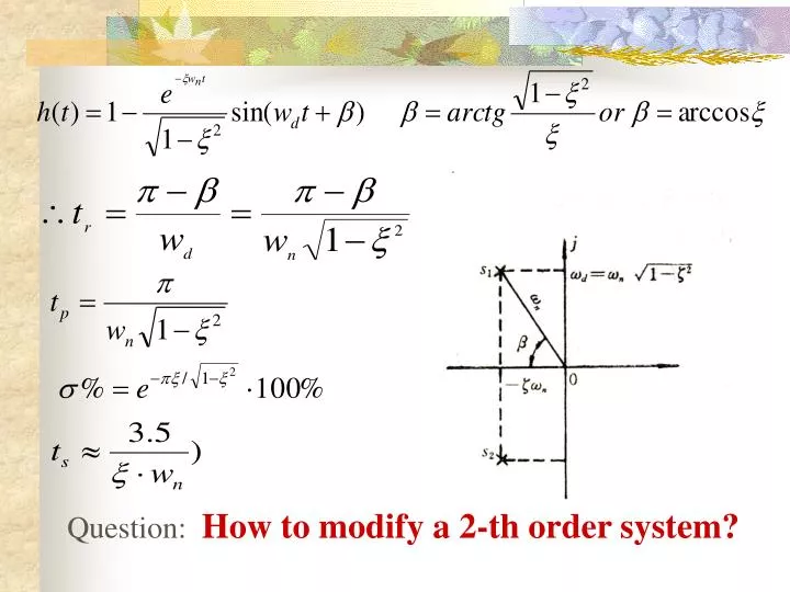
Question: How to modify a 2-th order system?. Exam.2. fig.: with a speed feedback 2th order system 。 Analyze the action of speed feedback 。 Open-loop TF. Closed-loop TF so , w n= constant, transient performance goes good. Equivalent damped ratio :.

E N D
Exam.2. fig.: with a speed feedback 2th order system。 Analyze the action of speed feedback 。 Open-loop TF
Closed-loop TF so ,wn=constant, transient performance goes good. Equivalent damped ratio :
When speed feedback is used, select appropriately kt, make ξincrease appropriately to decrease over-shoot, increase response speed, make the system satisfy all the requests.
Exam.3 following fig. is a 2th order system with proportion-differential control,output is controlled by deviation and its differential 。Analyze the action of proportion-differential correction。
Open-loop TF closed-loop TF : Equivalent damped ratio:
Duo to wn is a constanttoo, Equivalent damped ratio make the б% ↓,ts ↓.And, proportion-differential control adds system a closed loop zero s=-1/ Td, front calculation results are no longer appropriate.but in general,good transient performance can be reached.
Exam.4:given a unit feedback system.its open-loop TF requirements:ts=7, σ %=16% solve T,K.
Exam.5 (1) Fig.(b) σ%=16%,tp=1.14s,solve K and Kt; (2) Solve unit step response in fig. (a) and (b).
In fig (b), From σ%==16% tp=1.14s
4 high order system time domain response Which is higher than 2th order system.
When r(t)=1(t),that is When all the characteristic roots are real numbers
How to analyze a high order system: 1.Dominating poles: |pi|>5|pj| e-5pit decreases quicker than e-pit 2.couple poles Zeros and poles can be cancelled.
Dominating poles: |pi|>5|pj| e-5pit decreases quicker than e-pit
5. relation between step response and zeros and poles (1). relation between step response and zeros assume a closed loop negative real zero be added, its output changes to,
If an added zero in right s-plane, the response changes slower.In general ts ↑, σ% ↓ 。
(2). relation between step response and poles assume a closed loop negative real pole be added, its output changes to the response changes slower.In general ts ↑, σ% ↓ 。
Homework: 3-10
** 在MATLAB中数学模型的表示 控制系统的数学模型在系统分析和设计中是相当重要的,在线性系统理论中常用的数学模型有微分方程、传递函数、状态空间表达式等,而这些模型之间又有着某些内在的等效关系。MATLAB主要使用传递函数和状态空间表达式来描述线性时不变系统(Linear Time Invariant简记为LTI)。
单输入单输出线性连续系统的传递函数为 其中m≤n。G(s)的分子多项式的根称为系统的零点,分母多项式的根称为系统的极点。令分母多项式等于零,得系统的特征方程: *.1传递函数 D(s)=a0sn+a1sn-1+……+an-1s+an=0
因传递函数为多项式之比,所以我们先研究MATLAB是如何处理多项式的。MATLAB中多项式用行向量表示,行向量元素依次为降幂排列的多项式各项的系数,例如多项式P(s)=s3+2s+4 ,其输入为 >>P=[1 0 2 4] 注意尽管s2项系数为0,但输入P(s)时不可缺省0。 MATLAB下多项式乘法处理函数调用格式为 C=conv(A,B)
例如给定两个多项式A(s)=s+3和B(s)=10s2+20s+3,求C(s)=A(s)B(s),则应先构造多项式A(s)和B(s),然后再调用conv( )函数来求C(s) >>A =[1,3]; B =[10,20,3]; >>C = conv(A,B) C = 10 50 63 9 即得出的C(s)多项式为10s3+50s2 +63s +9
MATLAB提供的conv( )函数的调用允许多级嵌套,例如 G(s)=4(s+2)(s+3)(s+4) 可由下列的语句来输入 >>G=4*conv([1,2],conv([1,3],[1,4]))
有了多项式的输入,系统的传递函数在MATLAB下可由其分子和分母多项式唯一地确定出来,其格式为有了多项式的输入,系统的传递函数在MATLAB下可由其分子和分母多项式唯一地确定出来,其格式为 sys=tf(num,den) 其中num为分子多项式,den为分母多项式 num=[b0,b1,b2,…,bm];den=[a0,a1,a2,…,an];
对于其它复杂的表达式,如 可由下列语句来输入 >>num=conv([1,1],conv([1,2,6],[1,2,6])); >>den=conv([1,0,0],conv([1,3],[1,2,3,4])); >>G=tf(num,den) Transfer function:
传递函数G(s)输入之后,分别对分子和分母多项式作因式分解,则可求出系统的零极点,MATLAB提供了多项式求根函数roots(),其调用格式为传递函数G(s)输入之后,分别对分子和分母多项式作因式分解,则可求出系统的零极点,MATLAB提供了多项式求根函数roots(),其调用格式为 roots(p) *.2传递函数的特征根及零极点图 其中p为多项式。
例如,多项式p(s)=s3+3s2+4 >>p=[1,3,0,4]; %p(s)=s3+3s2+4 >>r=roots(p)%p(s)=0的根 r=-3.3533 0.1777+1.0773i 0.1777-1.0773i 反过来,若已知特征多项式的特征根,可调用MATLAB中的poly( )函数,来求得多项式降幂排列时各项的系数,如上例 >>poly(r) p = 1.0000 3.0000 0.0000 4.0000
而polyval函数用来求取给定变量值时多项式的值,其调用格式为而polyval函数用来求取给定变量值时多项式的值,其调用格式为 polyval(p,a) 其中p为多项式;a为给定变量值 例如,求n(s)=(3s2+2s+1)(s+4)在s=-5时值: >>n=conv([3,2,1],[1,4]); >>value=polyval(n,-5) value=-66
传递函数在复平面上的零极点图,采用pzmap()函数来完成,零极点图上,零点用“。”表示,极点用“×”表示。其调用格式为传递函数在复平面上的零极点图,采用pzmap()函数来完成,零极点图上,零点用“。”表示,极点用“×”表示。其调用格式为 [p,z]=pzmap(num,den) 其中, p─传递函数G(s)= numden的极点 z─传递函数G(s)= numden的零点 例如,传递函数
用MATLAB求出G(s)的零极点,H(s)的多项式形式,及G(s)H(s)的零极点图用MATLAB求出G(s)的零极点,H(s)的多项式形式,及G(s)H(s)的零极点图 >>numg=[6,0,1]; deng=[1,3,3,1]; >>z=roots(numg) z=0+0.4082i 0-0.4082i %G(s)的零点 >>p=roots(deng) p=-1.0000+0.0000i -1.0000+0.0000i %G(s)的极点 -1.0000+0.0000i
>> n1=[1,1];n2=[1,2];d1=[1,2*i]; d2=[1,-2*i];d3=[1,3]; >>numh=conv(n1,n2); denh=conv(d1,conv(d2,d3)); >>printsys(numh,denh) numh/denh= %H(s)表达式 >>pzmap(num,den) %零极点图 >>title(‘pole-zero Map’)
若已知控制系统的方框图,使用MATLAB函数可实现方框图转换。若已知控制系统的方框图,使用MATLAB函数可实现方框图转换。 1.串联 如图所示G1(s)和G2(s)相串联,在MATLAB中可用串联函数series( )来求G1(s)G2(s),其调用格式为 [num,den]=series(num1,den1,num2,den2) 其中: *.3 控制系统的方框图模型
2.并联 如图所示G1(s)和G2(s)相并联,可由MATLAB的并联函数parallel( )来实现,其调用格式为 [num,den]=parallel(num1,den1,num2,den2) 其中:
3.反馈 反馈连接如图所示。使用MATLAB中的feedback( )函数来实现反馈连接,其调用格式为 [num,den]=feedback(numg,deng,numh,denh,sign) 式中: sign为反馈极性,若为正反馈其为1,若为负反馈其为-1或缺省。
例如G(s)= ,H(s)= ,负反馈连接。 >>numg=[1,1];deng=[1,2]; >>numh=[1];denh=[1,0]; >>[num,den]=feedback(numg,deng,numh,denh,-1); >> printsys(num,den) num/den=
MATLAB中的函数series,parallel和feedback可用来简化多回路方框图。另外,对于单位反馈系统,MATLAB可调用cloop( )函数求闭环传递函数,其调用格式为 [num,den]=cloop(num1,den1,sign)
传递函数可以是时间常数形式,也可以是零极点形式,零极点形式是分别对原系统传递函数的分子和分母进行因式分解得到的。MATLAB控制系统工具箱提供了零极点模型与时间常数模型之间的转换函数,其调用格式分别为传递函数可以是时间常数形式,也可以是零极点形式,零极点形式是分别对原系统传递函数的分子和分母进行因式分解得到的。MATLAB控制系统工具箱提供了零极点模型与时间常数模型之间的转换函数,其调用格式分别为 [z,p,k]= tf2zp(num,den) [num,den]= zp2tf(z,p,k) *.4 控制系统的零极点模型 其中第一个函数可将传递函数模型转换成零极点表示形式,而第二个函数可将零极点表示方式转换成传递函数模型。
例如G(s)= 用MATLAB语句表示: >>num=[12241220];den=[24622]; >>[z,p,k]=tf2zp(num,den) z= -1.9294 -0.0353+0.9287i -0.0353-0.9287i
p=-0.9567+1.2272i -0.9567-1.2272i -0.0433+0.6412i -0.0433-0.6412i k=6 即变换后的零极点模型为 G(s)=
可以验证MATLAB的转换函数,调用zp2tf()函数将得到原传递函数模型。可以验证MATLAB的转换函数,调用zp2tf()函数将得到原传递函数模型。 >>[num,den]=zp2tf(z,p,k) num = 0 6.0000 12.0000 6.0000 10.0000 den = 1.0000 2.0000 3.0000 1.0000 1.0000 即
** 用MATLAB和SIMULINK进行瞬态响应分析 *.1 单位脉冲响应 当输入信号为单位脉冲函数δ(t)时,系统输出为单位脉冲响应,MATLAB中求取脉冲响应的函数为impulse( ),其调用格式为 [y,x,t]=impulse(num,den,t) 或 impulse(num,den) 式中G(s)=num/den; t为仿真时间; y为时间t的输出响应;x为时间t的状态响应。
例试求下列系统的单位脉冲响应 MATLAB命令为: >> t=[0:0.1:40]; >>num=[1]; >>den=[1,0.3,1]; >>impulse(num,den,t); >>grid; >>title('Unit-impulse Response of G(s)=1/(s^2+0.3s+1)') 其响应结果如图所示。