Download
1 / 48
490 likes | 730 Views
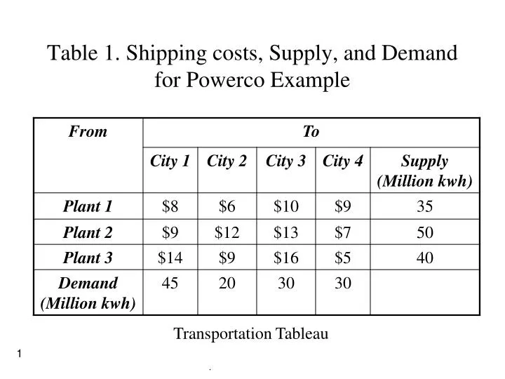
Table 1. Shipping costs, Supply, and Demand for Powerco Example. Transportation Tableau. Solution. Decision Variable: Since we have to determine how much electricity is sent from each plant to each city; X ij = Amount of electricity produced at plant i and sent to city j

E N D
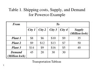
Table 1. Shipping costs, Supply, and Demand for Powerco Example Transportation Tableau
Solution Decision Variable: Since we have to determine how much electricity is sent from each plant to each city; Xij = Amount of electricity produced at plant i and sent to city j X14 = Amount of electricity produced at plant 1 and sent to city 4
2. Objective function Since we want to minimize the total cost of shipping from plants to cities; Minimize Z = 8X11+6X12+10X13+9X14 +9X21+12X22+13X23+7X24 +14X31+9X32+16X33+5X34
3. Supply Constraints Since each supply point has a limited production capacity; X11+X12+X13+X14 <= 35 X21+X22+X23+X24 <= 50 X31+X32+X33+X34 <= 40
4. Demand Constraints Since each supply point has a limited production capacity; X11+X21+X31 >= 45 X12+X22+X32 >= 20 X13+X23+X33 >= 30 X14+X24+X34 >= 30
5. Sign Constraints Since a negative amount of electricity can not be shipped all Xij’s must be non negative; Xij >= 0 (i= 1,2,3; j= 1,2,3,4)
LP Formulation of Powerco’s Problem Min Z = 8X11+6X12+10X13+9X14+9X21+12X22+13X23+7X24 +14X31+9X32+16X33+5X34 S.T.: X11+X12+X13+X14 <= 35 (Supply Constraints) X21+X22+X23+X24 <= 50 X31+X32+X33+X34 <= 40 X11+X21+X31 >= 45 (Demand Constraints) X12+X22+X32 >= 20 X13+X23+X33 >= 30 X14+X24+X34 >= 30 Xij >= 0 (i= 1,2,3; j= 1,2,3,4)
General Description of a Transportation Problem A set of m supply points from which a good is shipped. Supply point i can supply at most si units. A set of n demand points to which the good is shipped. Demand point j must receive at least di units of the shipped good. Each unit produced at supply point i and shipped to demand point j incurs a variable cost of cij.
Xij = number of units shipped from supply point i to demand point j
Balanced Transportation Problem If Total supply equals to total demand, the problem is said to be a balanced transportation problem:
Balancing a TP if total supply exceeds total demand If total supply exceeds total demand, we can balance the problem by adding dummy demand point. Since shipments to the dummy demand point are not real, they are assigned a cost of zero.
Balancing a transportation problem if total supply is less than total demand If a transportation problem has a total supply that is strictly less than total demand the problem has no feasible solution. There is no doubt that in such a case one or more of the demand will be left unmet. Generally in such situations a penalty cost is often associated with unmet demand and as one can guess this time the total penalty cost is desired to be minimum
Optimal solution is found as: X12=10, X13=25, X21=45, X23=5, X32=10, X34=30cost 1020
Assignment Problems Example: Machineco has four jobs to be completed. Each machine must be assigned to complete one job. The time required to setup each machine for completing each job is shown in the table below. Machinco wants to minimize the total setup time needed to complete the four jobs.
Setup times (Also called the cost matrix)
The Model According to the setup table Machinco’s problem can be formulated as follows (for i,j=1,2,3,4):
For the model on the previous page note that: Xij=1 if machine i is assigned to meet the demands of job j Xij=0 if machine i is not assigned to meet the demands of job j In general an assignment problem is balanced transportation problem in which all supplies and demands are equal to 1.
The Assignment Problem In general the LP formulation is given as Minimize Each supply is 1 Each demand is 1
Solution in the example • X(1,2)=1 • X(2,4)=1 • X(3,3)=1 • X(4,1)=1
Comments on the Assignment Problem • The Air Force has used this for assigning thousands of people to jobs. • This is a classical problem. Research on the assignment problem predates research on LPs. • Very efficient special purpose solution techniques exist. • 10 years ago, Yusin Lee and J. Orlin solved a problem with 2 million nodes and 40 million arcs in ½ hour.
Transshipment Problems A transportation problem allows only shipments that go directly from supply points to demand points. In many situations, shipments are allowed between supply points or between demand points. Sometimes there may also be points (called transshipment points) through which goods can be transshipped on their journey from a supply point to a demand point. Fortunately, the optimal solution to a transshipment problem can be found by solving a transportation problem.
Transshipment Example • Example 5: Widgetco manufactures widgets at two factories, one in Memphis and one in Denver. The Memphis factory can produce as 150 widgets, and the Denver factory can produce as many as 200 widgets per day. Widgets are shipped by air to customers in LA and Boston. The customers in each city require 130 widgets per day. Because of the deregulation of airfares, Widgetco believes that it may be cheaper first fly some widgets to NY or Chicago and then fly them to their final destinations. The cost of flying a widget are shown next. Widgetco wants to minimize the total cost of shipping the required widgets to customers.
Transportation Tableau Associated with the Transshipment Example • NY Chicago LA Boston Dummy Supply • Memphis $8 $13 $25 $28 $0 150 • Denver $15 $12 $26 $25 $0 200 • NY $0 $6 $16 $17 $0 350 • Chicago $6 $0 $14 $16 $0 350 • Demand 350 350 130 130 90 • Supply points: Memphis, Denver • Demand Points: LA Boston • Transshipment Points: NY, Chicago • The problem can be solved using the transportation simplex method
Maximum Flow Problem • Maximum flow problem description • All flow through a directed and connected network originates at one node (source) and terminates at one another node (sink) • All the remaining nodes are transshipment nodes • Flow through an arc is allowed only in the direction indicated by the arrowhead, where the maximum amount of flow is given by the capacity of that arc. At the source, all arcs point away from the node. At the sink, all arcs point into the node • The objective is to maximize the total amount of flow from the source to the sink (measured as the amount leaving the source or the amount entering the sink)
Maximum Flow Problem • Typical applications • Maximize the flow through a company’s distribution network from its factories to its customers • Maximize the flow through a company’s supply network from its vendors to its factories • Maximize the flow of oil through a system of pipelines • Maximize the flow of water through a system of aqueducts • Maximize the flow of vehicles through a transportation network
Maximum Flow Algorithm • Some Terminology • The residual network shows the remaining arc capacities for assigning additional flows after some flows have been assigned to the arcs The residual capacity for assigning some flow from node B to node O 5 2 O B The residual capacity for flow from node O to Node B
Maximum Flow Algorithm • An augmenting path is a directed path from the source to the sink in the residual network such that every arc on this path has strictly positive residual capacity • The residual capacity of the augmenting path is the minimum of these residual capacities (the amount of flow that can feasibly be added to the entire path) • Basic idea • Repeatedly select some augmenting path and add a flow equal to its residual capacity to that path in the original network. This process continues until there are no more augmenting paths, so that the flow from the source to the sink cannot be increased further
Maximum Flow Algorithm • The Augmenting Path Algorithm • Assume that the arc capacities are either integers or rational numbers • 1. identify an augmenting path by finding some directed path from the source to the sink in the residual network such that every arc on this path has strictly positive residual capacity. If no such path exists, the net flows already assigned constitute an optimal flow pattern • 2. Identify the residual capacity c* of this augmenting path by finding the minimum of the residual capacities of the arcs on this path. Increase the flow in this path by c*
Maximum Flow Example • During the peak season the park management of the Seervada park would like to determine how to route the various tram trips from the park entrance (Station O) to the scenic (Station T) to maximize the number of trips per day. Each tram will return by the same route it took on the outgoing trip so the analysis focuses on outgoing trips only. To avoid unduly disturbing the ecology and wildlife of the region, strict upper limits have been imposed on the number of outgoing trips allowed per day in the outbound direction on each individual road. For each road the direction of travel for outgoing trips is indicated by an arrow in the next slide. The number at the base of the arrow gives the upper limit on the number of outgoing trips allowed per day.
Maximum Flow Example (0,3) • Consider the problem of sending as many units from node O to node T for the following network (current flow, capacity): A D (0,9) (0,5) (0,1) T (0,4) (0,1) (0,7) O B (0,6) (0,5) (0,4) (0,2) E (0,4) C
Maximum Flow Example (0,3) • Iteration 1: one of the several augmenting paths is OBET, which has a residual capacity of min{7, 5, 6} = 5. By assigning the flow of 5 to this path, the resulting network is shown above A D (0,9) (0,5) (0,1) T (0,4) (0,1) (5,7) O B (5,6) (5,5) (0,4) (0,2) E (0,4) C
Maximum Flow Example (3,3) • Iteration 2: Assign a flow of 3 to the augmenting path OADT. The resulting residual network is A D (3,9) (3,5) (0,1) T (0,4) (0,1) (5,7) O B (5,6) (5,5) (0,4) (0,2) E (0,4) C
Maximum Flow Example (3,3) • Iteration 3: Assign a flow of 1 to the augmenting path OABDT. The resulting residual network is A D (4,9) (4,5) (1,1) T (1,4) (0,1) (5,7) O B (5,6) (5,5) (0,4) (0,2) E (0,4) C
Maximum Flow Example (3,3) • Iteration 4: Assign a flow of 2 to the augmenting path OBDT. The resulting residual network is A D (6,9) (4,5) (1,1) T (3,4) (0,1) (7,7) O B (5,6) (5,5) (0,4) (0,2) E (0,4) C
Maximum Flow Example (3,3) Iteration 5: Assign a flow of 1 to the augmenting path OCEDT. The resulting residual network is A D (7,9) (4,5) (1,1) T (3,4) (1,1) (7,7) O B (5,6) (5,5) (1,4) (0,2) E (1,4) C
Maximum Flow Example (3,3) Iteration 6: Assign a flow of 1 to the augmenting path OCET. The resulting residual network is A D (7,9) (4,5) (1,1) T (3,4) (1,1) (7,7) O B (6,6) (5,5) (2,4) (0,2) E (2,4) C
Maximum Flow Example • There are no more flow augmenting paths, so the current flow pattern is optimal 3 A 7 D 1 4 T 13 3 1 O B 13 6 7 5 E 2 C 2
Minimum Spanning Tree Problems Suppose that each arc (i,j) in a network has a length associated with it and that arc (i,j) represents a way of connecting node i to node j. For example, if each node in a network represents a computer in a computer network, arc(i,j) might represent an underground cable that connects computer i to computer j. In many applications, we want to determine the set of arcs in a network that connect all nodes such that the sum of the length of the arcs is minimized. Clearly, such a group of arcs contain no loop.
Minimum Spanning Tree Problem • An undirected and connected network is being considered, where the given information includes some measure of the positive length (distance, cost, time, etc.) associated with each link • Both the shortest path and minimum spanning tree problems involve choosing a set of links that have the shortest total length among all sets of links that satisfy a certain property • For the shortest-path problem this property is that the chosen links must provide a path between the origin and the destination • For the minimum spanning tree problem, the required property is that the chosen links must provide a path between each pair of nodes
Some Applications • Design of telecommunication networks (fiber-optic networks, computer networks, leased-line telephone networks, cable television networks, etc.) • Design of lightly used transportation network to minimize the total cost of providing the links (rail lines, roads, etc.) • Design of a network of high-voltage electrical transmission lines • Design of a network of wiring on electrical equipment (e.g., a digital computer system) to minimize the total length of the wire • Design of a network of pipelines to connect a number of locations
12 1 2 (1,2)-(2,3)-(3,1) is a loop 4 For a network with n nodes, a spanning tree is a group of n-1 arcs that connects all nodes of the network and contains no loops. 7 (1,3)-(2,3) is the minimum spanning tree 3
Minimum Spanning Tree Problem Description • You are given the nodes of the network but not the links. Instead you are given the potential links and the positive length for each if it is inserted into the network (alternative measures for length of a link include distance, cost, and time) • You wish to design the network by inserting enough links to satisfy the requirement that there be a path between every pair of nodes • The objective is to satisfy this requirement in a way that minimizes the total length of links inserted into the network
Minimum Spanning Tree Algorithm • Greedy Algorithm • 1. Select any node arbitrarily, and then connect (i.e., add a link) to the nearest distinct node • 2. Identify the unconnected node that is closest to a connected node, and then connect these two nodes (i.e., add a link between them). Repeat the step until all nodes have been connected • 3. Tie breaking: Ties for the nearest distinct node (step 1) or the closest unconnected node (step 2) may be broken arbitrarily, and the algorithm will still yield an optimal solution. • Fastest way of executing algorithm manually is the graphical approach illustrated next
1 1 2 2 2 6 5 4 3 2 4 4 3 5 Example: The State University campus has five computers. The distances between computers are given in the figure below. What is the minimum length of cable required to interconnect the computers? Note that if two computers are not connected this is because of underground rock formations.
1 1 2 2 Solution: We want to find the minimum spanning tree. Iteration 1: Following the MST algorithm discussed before, we arbitrarily choose node 1 to begin. The closest node is node 2. Now C={1,2}, Ć={3,4,5}, and arc(1,2) will be in the minimum spanning tree. 2 6 5 4 3 2 4 4 3 5
1 1 2 2 Iteration 2: Node 5 is closest to C. since node 5 is two blocks from node 1 and node 2, we may include either arc(2,5) or arc(1,5) in the minimum spanning tree. We arbitrarily choose to include arc(2,5). Then C={1,2,5} and Ć={3,4}. 2 6 5 4 3 2 4 4 3 5
1 1 2 2 Iteration 3: Since node 3 is two blocks from node 5, we may include arc(5,3) in the minimum spanning tree. Now C={1,2,5,3} and Ć={4}. 2 6 5 4 3 2 4 4 3 5
1 1 2 2 Iteration 4: Node 5 is the closest node to node 4. Thus, we add arc(5,4) to the minimum spanning tree. We now have a minimum spanning tree consisting of arcs(1,2), (2,5), (5,3), and (5,4). The length of the minimum spanning tree is 1+2+2+4=9 blocks. 2 6 5 4 3 2 4 4 3 5