Download
1 / 40
400 likes | 546 Views
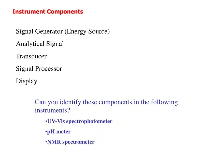
Instrument Components. Signal Generator (Energy Source) Analytical Signal Transducer Signal Processor Display. Can you identify these components in the following instruments? UV-Vis spectrophotometer pH meter NMR spectrometer.

E N D
Instrument Components Signal Generator (Energy Source) Analytical Signal Transducer Signal Processor Display • Can you identify these components in the following instruments? • UV-Vis spectrophotometer • pH meter • NMR spectrometer
Signal - the net response when a measurement is performed. It consists of several components (baseline, blank, noise) that must be subtracted from the response to determine the true analytical signal. Noise - the random excursion of the signal about some average value. If there is a lot of noise, then the signal becomes harder to measure. Signal-to-noise ratio (SNR) is frequently the most important parameter to optimize in any measurement system.
Types of noise Shot and thermal noise are consequences of properties of matter and cannot be avoided. They are distributed evenly at ALL frequencies and are referred to as white noise. Flicker noise is more intense at low frequencies than high frequencies, varying approximately as 1/f and is only appreciable below 1 KHz. Environmental noise is usually the dominant source arising primarily from 60 Hz transmission lines (and higher harmonics). Other sources of environmental noise include vibrations and electrical interactions between instruments.
Intuitively, the relative amounts of signal and noise will influence the precision associated with the measurement. Our confidence in a measurement performed in a high-noise environment differs from that in a low-noise environment. In the lab, if the results of an experiment are noisy, one typically replicates the experiment and reports the mean or average result. In fact, the mean of many measurements will more accurately estimate the true signal.
Boxcar Averaging The average (or sum) of a set of points replaces the individual values over a narrow portion of the data set. This operation is repeated over the entire domain of data. interval } Original data set } Boxcar averaged data set
Boxcar Averaging Number of points in interval Nbox= 1
Boxcar Averaging Nbox= 3
Boxcar Averaging Nbox= 5
Boxcar Averaging Nbox= 7
Boxcar Averaging Nbox= 11
Boxcar Averaging • Limitations of boxcar averaging: • Analysis time increases. • Resolution decreases. * • Distortion increases. * • Number of points per data set reduced by a factor of N. • Time-dependent information is maintained.
Moving Average Number of points in moving window Nmov box = 1
Moving Average Nmov box= 3
Moving Average Nmov box= 5
Moving Average Nmov box= 7
Moving Average Nmov box= 9
Moving Average Nmov box= 15
Moving Average Nmov box= 25
Moving Average • Limitations of moving average: • Analysis time increases. • Resolution decreases. * • Distortion increases. * • Time-dependent information is maintained.
Savitsky-Golay Smoothing A polynomial is fit to the data in each window. The center value is replaced by the calculated value from the model. The window is shifted and the fitting process is repeated. Savitsky and Golay developed a set of weighting factors (integers) that, when used in a convolution process, and achieve the same effect as as a least squares fit to a polynomial equation, but in a faster, neater, and more elegant manner.
Savitsky-Golay Smoothing Number of points in moving window Nmov box = 1
Savitsky-Golay Smoothing Nmov box= 5
Savitsky-Golay Smoothing Nmov box= 7
Savitsky-Golay Smoothing Nmov box= 9
Savitsky-Golay Smoothing Nmov box= 13
Savitsky-Golay Smoothing Nmov box= 17
Savitsky-Golay Smoothing Nmov box= 19
Savitsky-Golay Smoothing • Limitations of Savitsky-Golay smoothing: • Analysis time increases. • Resolution decreases. * • Distortion increases. * • Time-dependent information is maintained.
Moving Average Savitsky-Golay Smoothing Nmov box= 15 Nmov box= 19 Which method yields the better SNR? Which provides lower distortion?
Ensemble Averaging Number of averaged data sets Ne.a. = 1 Point by point ensemble averaging should increase the SNR by the square root of N. Let’s check it out….
Ensemble Averaging Ne.a. = 10
Ensemble Averaging Ne.a. = 20
Ensemble Averaging Ne.a. = 50
Ensemble Averaging Ne.a. = 100
Ensemble Averaging Ne.a. = 200
Ensemble Averaging Ne.a. = 1000
Ensemble Averaging • Limitations of ensemble averaging: • Repetitive measurement of the same sample is required. • Time per experiment increases by a factor of N. • Time-dependent information is lost. You can not tell if there is a drift, or systematic error in the data with only the average. • SNR is dramatically improved with minimal distortion.
Digital Filtering To remove interference noise, the following process is employed: 1. Time-domain data is transformed into frequency-domain data with the Fourier transform. 2. Selected frequencies are deleted (or multiplied by filtering function) 3. The digitally filtered frequency-domain data back to the time-domain using the inverse Fourier transform.