Download
1 / 20
200 likes | 305 Views
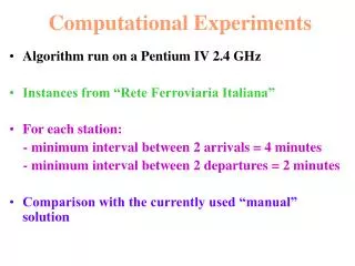
Computational Experiments. Algorithm run on a Pentium IV 2.4 GHz Instances from “Rete Ferroviaria Italiana” For each station: - minimum interval between 2 arrivals = 4 minutes - minimum interval between 2 departures = 2 minutes Comparison with the currently used “manual” solution.

E N D
Computational Experiments • Algorithm run on a Pentium IV 2.4 GHz • Instances from “Rete Ferroviaria Italiana” • For each station: - minimum interval between 2 arrivals = 4 minutes - minimum interval between 2 departures = 2 minutes • Comparison with the currently used “manual” solution
The “shift” and the “stretch” penalties are linear in the shift vj and in the stretch uj, respectively • Profit of train j = πj – αjvj – βj uj (ujand vj in minutes)
Additional Characteristics • Fixed block signalling • The line is divided into block sections of predetermined length • Each block section is occupied by at most one train at a time • Short sections are designed to increase line capacity, particularly in high density areas and where speeds are lower • Moving block signalling • The position of each train is known continuously by a control center, that takes care of the regulation of the relative distances • Modern technology that requires an efficient communication system between line signals, cabs and control centers
Additional Characteristics (2) • Capacities of the Stations • The maximim number of trains that can be simultaneously present in each station is given • Computational experiments: - capacity = 2 in the major stations - capacity = 1 in the minor stations
Addition of new train paths to an existing timetable (operational scenario) Example: single one-way track Kufstein – Verona: number of stations: 56 (345 km) - number of already scheduled trains: 230 (passenger trains 116, freight trains 114) - time frame period: from 00:00 to 23:59
Addition of new freight train paths to an existing timetable (Kufstein- Verona): Example 1) number of requested train paths: 24 (requested departure times with a delay of 5 minutes with respect to an existing path; conflicts among the new paths) maximum shift for each requested train = 10 min maximum stretch = 15 min: # scheduled trains = 11 maximum stretch = 20 min: # scheduled trains = 17 maximum stretch = 25 min: # scheduled trains = 20 maximum stretch = 30 min: # scheduled trains = 22 Running time 18 seconds
Addition of new freight train paths to an existing timetable (Kufstein- Verona): Example 2) number of requested train paths: 24 (requested departure times at 00:00, 01:00, …, 23:00) maximum shift for each requested train = 10 min maximum stretch = 15 min: # scheduled trains = 11 maximum stretch = 20 min: # scheduled trains = 15 maximum stretch = 25 min: # scheduled trains = 19 maximum stretch = 30 min: # scheduled trains = 21 Running time 11 seconds
Addition of new freight train paths to an existing timetable (Kufstein- Verona): Example 3) number of requested train paths: 48 (requested departure times at 00:00, 00:30, 01:00, …, 23:30) maximum shift for each requested train = 10 min maximum stretch = 15 min: # scheduled trains = 25 maximum stretch = 20 min: # scheduled trains = 33 maximum stretch = 25 min: # scheduled trains = 39 maximum stretch = 30 min: # scheduled trains = 45 Running time 13 seconds
Railway Network • The considered Railway Network is composed by: • the single one-way corridor Kufstein – Verona Porta Nuova • the corridor Verona Porta Nuova – Bologna (which presents double-way line segments) • the railway node of Bologna • the alternative routes from Bologna to Rome (Florence and Falconara) • the railway node of Florence • the different possible routes from Florence to Rome ( “direttissima”, i.e. the fast line and, “lenta”, i.e. the slow line) • the railway node of Rome
We start with a feasible timetable with 679 fixed trains and evaluate two different cases of adding new freight trains: • 24 trains, one each hour • 48 trains, one each half an hour • For both cases, we consider two different possibilities: • forbid the alternative slow route (Falconara route) • allow to use the slow route (Falconara route) • Moreover, we consider different values of the maximum stretch.
The table shows the number of scheduled trains if the Falconara route cannot be used.
The table shows the number of scheduled trains if the Falconara route is allowed.
Overall Advantages of the • Optimization Algorithms • Much faster response time with respect to “manual” methods, with the possibility to try several different scenarios • Improvement of the solution quality with respect to “manual” methods • Satisfaction of a larger number of TO requests • Possibility to handle more than one request in “real time”