Introduction to Hidden Markov Model

1. Introduction to Hidden Markov Model Alexandre Savard March 2006

2. Overview • Introduction • Discrete Markov process • Extension to Hidden Markov Model • Three Fundamental Problems • Evaluation of the probability of a sequence of observation • The determination of a best sequence of model state • Adjustment of model parameters so as to best account for the observed signal • Interesting Website • Conclusion

3. Introduction • Definition of Signal Model • Deterministic Model • One dimensional wave equation • Simple harmonic pendulum • Statistical Model • Gaussian process • Poisson process • Markov process • Hidden Markov Model

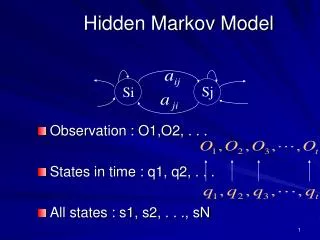
4. Discrete Markov Process • Theory of Markov Model • We consider a set of N distinct states of a system : • The system undergoes • a change of state according • to a set of probabilities • associated with the states Rabiner L., A tutorial on Hidden Markov models and selected application in speech recognition

5. Discrete Markov Process • Theory of Markov Model • We denote the time instants associated with state changes as : • We denote the actual state at time t as : • A Markov chain of order M is a probabilistic description involving the current state and the M previous states • The state transition probabilities for first order chain:

6. Discrete Markov Process • Assumption in the theory • In the case of a first order model, it is assumed that the current state is only dependant upon the previous state. • It is assumed that state transition probabilities are independent of the actual time at which the transition takes place. • It is assumed that current observation is statistically independent of the previous observations.

7. Discrete Markov Process • Example of Markov Model • State 1 : Rainy State 2 : Cloudy state 3 : Sunny • Transition probability matrix (Model) : • Initial state probabilities : • Observation sequence :

8. Discrete Markov Process • Example of Markov Model • Given that model, what are the probability to get the given observation :

9. Hidden Markov Models • Extension to Hidden Markov Model • So far we have considered Markov models in which each state correspond to an observable event • This model is too restrictive to be applicable to many problems of interest • We extend the concept to include the case where the observation is function of the state • Hidden Markov Model is a stochastic process with an underlying stochastic process that is not observable

10. Hidden Markov Models The Urn Ball model Rabiner L., A tutorial on Hidden Markov models and selected application in speech recognition

11. Hidden Markov Models • Element of an HMM • N, the n umber of state in the model. Generally, the state are interconnected in such a way that any state can be reached from any other state. • M, the number of distinct observation symbols per state. We denote the individual symbol as :

12. Hidden Markov Models • Element of an HMM • The state transition distribution • The observation symbol probability distribution in state j • The initial state distribution

13. Hidden Markov Models • HMM Requirement • Specification of two model parameters (N and M) • Specification of observation symbols • Specification of the three probability measures

14. Three Fundamental Problems • Problems for HMMs • Given the observation sequence O and a model , how do we efficiently compute P(O|), the probability of the observation sequence according to the model ? • Given the observation sequence O and a model , how do we choose a corresponding state sequence Q which is optimal in some meaningful sense (best explains the observations) ? • How do we adjust the model parameters  to maximize P(O|) ?

15. Three Fundamental Problems • Problem 1: Evaluation Problem • How do we compute the probability that the observed sequence was produced by the model ? • Consider one such fixed state sequence and its probability: • The probability of the observation sequence of Q is:

16. Three Fundamental Problems • Problem 1: Evaluation Problem • The probability that O and Q occur simultaneously is • The probability of O is obtain by summing this joint probability over all state sequence q • It needs (2T - 1) N^T multiplication and N^T-1 addition

17. Three Fundamental Problems • Problem 1: Forward/Backward Process • Consider the forward variable  that evaluates the probability of a partial observation sequence up to time t • We can solve for  inductively

18. Three Fundamental Problems • Problem 1: Forward/Backward Process • In a same way we can define a backward variable that gives the probabilities from t + 1 to the end • We can solve for  inductively

19. Three Fundamental Problems • Problem 2: Decoding Problem • It is the one in which we attempt to uncover the hidden part of the model, to find the correct state sequence. • We usually use an optimality criterion to solve this problem. • The most widely used criterion is to find the single best sequence that maximizes P(Q|O,).

20. Three Fundamental Problems • Problem 2: Decoding Problem • We define , the probability of being in state S at time t, given the observations O and the model  •  accounts for the partial observation sequence •  accounts for the remainder observation sequence

21. Three Fundamental Problems • Problem 2: Decoding Problem • Using  we can solve for the most likely state for each time t • Some times this method does not give a physically meaningful state sequence

22. Three Fundamental Problems • Problem 2: Viterbi Algorithm • We need to define the quantity  that accounts for the first t observation • By mathematical induction we have

23. Three Fundamental Problems • Problem 2: Viterbi Algorithm • Instead of looking to a localized optimization of the probabilities for each observation, we try to find the overall path that maximises the probabiliy. http://www.comp.leeds.ac.uk/roger/HiddenMarkovModels/html_dev/viterbi_algorithm/s1_pg11.html

24. Three Fundamental Problems • Problem 3: Training Problem • We attempt to optimize the model parameters so as to best describe how a given observation sequence comes about • There is no known analytical way to solve for the model that maximizes the probabilities • The optimizations process can be different from application to application • We can however choose  such that P(O| ) is locally maximized using an iterative procedure.

25. Three Fundamental Problems • Problem 3: Baum-Welch Algorithm • We define  the probability of being in a given state at time t and in an other specific one at time t + 1

26. Three Fundamental Problems • Problem 3: Baum-Welch Algorithm • We define  the probability of being in a specific state at time t given an observation sequence O and a model  • Summing  over the time index t we get the expected number of transition between the two states • Summing  over t, we get the number of time a specific state is visited

27. Three Fundamental Problems • Problem 3: Baum-Welch Algorithm • We can then define the optimized model as:

28. Three Fundamental Problems • Problem 3: Other Algorithms • Maximum Likelihood criterion • Baum-Welch Algorithm • Gradient based method • Maximum Mutual information criterion • Gradient wrt transition probabilities • Gradient wrt observation probabilities

29. Internet Links • Interesting website concerning HMM • Learning about Hidden Markov Model • http://jedlik.phy.bme.hu/~gerjanos/HMM/node2.html • Free library available on the web • Library in Matlab • http://www.cs.ubc.ca/~murphyk/Software/HMM/hmm.html • Library in Java • http://www.run.montefiore.ulg.ac.be/~francois/software/jahmm/

30. Conclusion

31. Bibliography • Rabiner L. 1989. A tutorial on Hidden Markov Models and selected applications in speech recognition. Proceedings of the IEEE, vol. 77, no. 2.