Download

1 / 22
230 likes | 268 Views
Stanley Chang OPLAB. Hidden Markov Model. Agenda. Introduction Hidden Markov Model (HMM) Markov Process Hidden Markov Model Applications of Hidden Markov Model. Introduction. Hidden Markov Model (intro.). A statistical model

E N D
Stanley Chang OPLAB Hidden Markov Model
Agenda • Introduction • Hidden Markov Model (HMM) • Markov Process • Hidden Markov Model • Applications of Hidden Markov Model OPLAB
Introduction OPLAB
Hidden Markov Model (intro.) • A statistical model • First described in a series of statistical papers by Leonard E. Baum and other authors in 1960s • The system being modeled is assumed to be a Markov process with unknown parameters • The challenge is to determine the hidden parameters from the observable parameters OPLAB
Markov Process • An Example: Stock Market Index 0.2 0.6 0.3 Bull Bear 0.5 up down 0.2 0.4 0.1 0.2 Even 0.5 unchanged OPLAB
Markov Process (cont.) • Three states: • Bull, Bear and Even • Three index observations: • Up, Down and Unchanged • The model is a Finite State Machine • With probabilistic transitions between states • Up-Down-Down → Bull-Bear-Bear • the probability of the sequence is simply the product of the transitions, 0.2 × 0.3 × 0.3 OPLAB
Markov Process (cont.) • Formal Definition: • A random process: • state at time t is X(t), for t > 0 • history of states is given by x(s) for times s < t is a Markov process if: • Future state is independent of its past states OPLAB
Hidden Markov Model OPLAB
Hidden Markov Model Example • Extend previous model into HMM: 0.2 0.6 0.3 up up Bull Bear 0.1 0.7 down 0.6 down 0.1 0.2 0.3 0.5 unchanged unchanged 0.2 0.4 0.1 0.2 Even up 0.3 0.3 down 0.4 0.5 unchanged OPLAB
Hidden Markov Model Example (cont.) • Same model: Bull Bear Even up down unchanged OPLAB
Hidden Markov Model Example (cont.) • Key difference: • if we have the observation sequence up-down-down… • we cannot say exactly what state sequence produced these observations • thus the state sequence is ‘hidden’ OPLAB
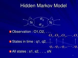
Hidden Markov Model • General architecture: • x(t) is the hidden state at time t • random variable y(t) is the observation at time t x(t-1) x(t) x(t+1) …… …… y(t-1) y(t) y(t+1) OPLAB
Hidden Markov Model (cont.) • the value of the hidden variable x(t) only depends on the value of the hidden variable x(t − 1) • The values at time t − 2 and before have no influence • the value of the observed variable y(t) only depends on the value of the hidden variable x(t) • Markov property OPLAB
Hidden Markov Model (cont.) • Formal definition: λ = (A,B,π) • State set: S = (s1, s2, · · · , sN) • Observation set: V = (v1, v2, · · · , vM) • Define Qto be a fixed state sequence of length T, and corresponding observations O • Q = q1, q2, · · · , qT • O = o1, o2, · · · , oT OPLAB
Hidden Markov Model (cont.) • Transition array A, storing the probability of state j following state i • A = [aij ] , aij = P(qt = sj | qt−1 = si) • Observation array B, storing the probability of observation k being produced from the state j • B = [bi(k)] , bi(k) = P(xt = vk | qt = si) • Initial probability array π • π = [πi] , πi = P(q1 = si) OPLAB
Hidden Markov Model (cont.) Two assumptions are made by the model: • Markov assumption: • the current state is dependent only on the previous state • P(qt | q1t-1) = P(qt | qt-1) • independence assumption: • the output observation at time t is dependent only on the current state, it is independent of previous observations and states • P(ot | o1t-1, q1t) = P(ot | qt) OPLAB
Variation of HMM Problem - 1 • Given: parameters of the model • Compute: • probability of a particular output sequence • probabilities of the hidden state values given that output sequence • Solved by the forward-backward algorithm OPLAB
Variation of HMM Problem - 2 • Given: parameters of the model • Find: the most likely sequence of hidden states that could have generated a given output sequence • Solved by the Viterbi algorithm OPLAB
Variation of HMM Problem - 3 • Given: output sequence (or a set of such sequences) • Find: the most likely set of state transition and output probabilities • Given a dataset of sequences, discover the parameters of the HMM • solved by the Baum-Welch algorithm OPLAB
Applications of HMM • Speech recognition (1970s) • Cryptanalysis • Machine translation • Partial discharge • Gene prediction • 行動通訊中節點移動的樣式 • 網路攻擊模式 • 殭屍網路流量行為之早期偵測 • …… OPLAB