Download
1 / 35
350 likes | 560 Views
Hidden Markov Model. Observation : O1,O2, . . . States in time : q1, q2, . . . All states : s1, s2, . . ., sN. Sj. Si. Hidden Markov Model (Cont’d). Discrete Markov Model. Degree 1 Markov Model. Hidden Markov Model (Cont’d). : Transition Probability from Si to Sj , .

E N D
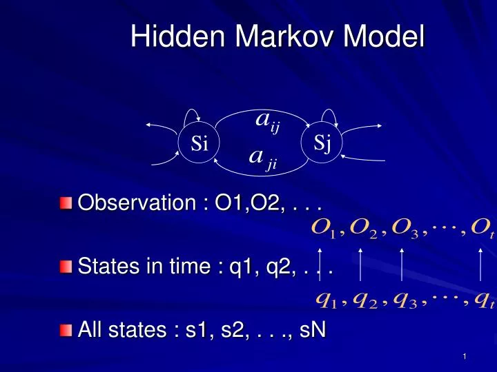
Hidden Markov Model • Observation : O1,O2, . . . • States in time : q1, q2, . . . • All states : s1, s2, . . ., sN Sj Si
Hidden Markov Model (Cont’d) • Discrete Markov Model Degree 1 Markov Model
Hidden Markov Model (Cont’d) : Transition Probability from Si to Sj ,
Discrete Markov Model Example S1 : The weather is rainy S2 : The weather is cloudy S3 : The weather is sunny cloudy sunny rainy rainy cloudy sunny
Hidden Markov Model Example (Cont’d) Question 1:How much is this probability: Sunny-Sunny-Sunny-Rainy-Rainy-Sunny-Cloudy-Cloudy
Hidden Markov Model Example (Cont’d) The probability of being in state i in time t=1 Question 2:The probability of staying in state Si for d days if we are in state Si? d Days
Discrete Density HMM Components • N : Number Of States • M : Number Of Outputs • A (NxN) : State Transition Probability Matrix • B (NxM): Output Occurrence Probability in each state • (1xN): Initial State Probability : Set of HMM Parameters
Three Basic HMM Problems • Recognition Problem: Given an HMM and a sequence of observations O,what is the probability ? • State Decoding Problem: Given a model and a sequence of observations O, what is the most likely state sequence in the model that produced the observations? • Training Problem: Given a model and a sequence of observations O, how should we adjust model parameters in order to maximize ?
First Problem Solution We Know That: And
First Problem Solution (Cont’d) Computation Order :
Forward Backward Approach Computing 1) Initialization
Forward Backward Approach (Cont’d) 2) Induction : 3) Termination : Computation Order :
Backward Variable 1) Initialization 2)Induction
Second Problem Solution • Finding the most likely state sequence Individually most likely state :
Viterbi Algorithm • Define : P is the most likely state sequence with this conditions : state i , time t and observation o
Viterbi Algorithm (Cont’d) 1) Initialization Is the most likely state before state i at time t-1
Viterbi Algorithm (Cont’d) 2) Recursion
Viterbi Algorithm (Cont’d) 3) Termination: 4)Backtracking:
Third Problem Solution • Parameters Estimation using Baum-Welch Or Expectation Maximization (EM) Approach Define:
Third Problem Solution (Cont’d) : Expected value of the number of jumps from state i : Expected value of the number of jumps from state i to state j
Baum Auxiliary Function By this approach we will reach to a local optimum
Continuous Observation Density • We have amounts of a PDF instead of • We have Mixture Coefficients Variance Average
Continuous Observation Density • Mixture in HMM M1|1 M1|2 M1|3 M2|1 M2|2 M2|3 M3|1 M3|2 M3|3 M4|1 M4|2 M4|3 S2 S3 S1 Dominant Mixture:
Continuous Observation Density (Cont’d) • Model Parameters: N×M×K×K 1×N N×M N×M×K N×N N : Number Of States M : Number Of Mixtures In Each State K : Dimension Of Observation Vector
Continuous Observation Density (Cont’d) Probability of event j’th state and k’th mixture at time t
State Duration Modeling Sj Si Probability of staying d times in state i :
State Duration Modeling (Cont’d) HMM With clear duration ……. ……. Sj Si
State Duration Modeling (Cont’d) • HMM consideration with State Duration : • Selecting using ‘s • Selecting using • Selecting Observation Sequence using in practice we assume the following independence: • Selecting next state using transition probabilities . We also have an additional constraint:
Training In HMM • Maximum Likelihood (ML) • Maximum Mutual Information (MMI) • Minimum Discrimination Information (MDI)
Training In HMM • Maximum Likelihood (ML) . . . Observation Sequence
Training In HMM (Cont’d) • Maximum Mutual Information (MMI) Mutual Information
Training In HMM (Cont’d) • Minimum Discrimination Information (MDI) Observation : Auto correlation :