Lecture 2 Hidden Markov Model

1. Lecture 2Hidden Markov Model

2. Hidden Markov Model Motivation: We have a text partly written by Shakespeare and partly “written” by a monkey, we want to write a program that can tell the which part was written by Shakespeare and which part by the monkey .

3. 21 century human-like monkey typing

4. Review on Probabilities • Probability of event X occurring is P(X) • Conditional probability • P(X|Y) : the probability of X occurring given Y • Joint probability • P(X,Y) = P(X|Y)P(Y) • P(X,Y|Z) = P(X|Y,Z)P(Y|Z) • Marginal probability • P(X) = SY P(X|Y)P(Y)

5. Posterior Probability • Usually we want to know probability of observationO given supposition (model) M; P(O|M) • Reverse problem: given O we want to know probability that M is correct: the posterior probability P(M|O) • Baye’s theorem: for any two event X, Y • P(X|Y) = P(Y|X)P(X)/P(Y) • P(M|O) = P(O|M)P(M)/P(O)

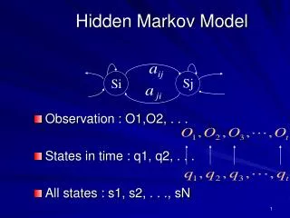
6. The Hidden Markov Model (HMM) is a finite set of states, each of which is associated with a probability distribution. Transitions among the states are governed by a set of probabilities called transition probabilities. In a particular state an outcome or observation can be generated, according to the associated probability distribution. It is only the outcome, not the state visible to an external observer and therefore states are ``hidden''from the observer; hence the name Hidden Markov Model. Definition of Hidden Markov Model

7. Examples • Text written by Shakespeare and monkey • Dice thrown by a dealer with two dice, one fair and one loaded • A DNA sequence with coding and non-coding segments

8. Examples (cont’d) Case Observed Hidden state symbols Text alphabet Shakespeare/monkey Dice 1-6 (rolled fair dice/loaded dice numbers) DNA A,C,G,T coding/non-coding (bases)

9. In order to define an HMM completely, following elements are needed. • The number of states of the model, {qi|i=1,2,..,N}. • The number of observation symbols in the alphabet, {ok |k=1,2,…,M}. • A set of state transition probabilities • where qt denotes the current state. • Transition probabilities should satisfy the • normal stochastic constraints, • and A

10. A emission probability distribution in each of the states, • where nk denotes the kth observation symbol in • the alphabet, and ot the current parameter vector. • Following stochastic constraints must be satisfied • and B bj(k) is the probability of state j taking the symbol nk

11. The initial state distribution, , where • Therefore we can use the compact notation • l = (A,B,p) • to denote an HMM with discrete probability distributions. Notation Sequence of observations: O = o1, o2, …, oT Sequence of (hidden) states: Q = q1, q2, …, qT

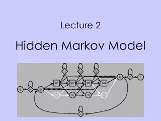
12. HMM scheme with K (DNA 4/protein 20) symbols © 2001 Per Kraulis [Mx] Match state x. Has K emission probabilities. [Dx ] Delete state x. Non-emitter. [Ix ] Insert state x. Has K emission probabilities. [B] Begin state (for entering main model). Non-emitter. [E] End state (for exiting main model). [S] Start state. Non-emitter. [N] N-terminal unaligned sequence state. Emits on transition with K emission probabilities. Non-emitter. [C] C-terminal unaligned sequence state. Emits on transition with K emission probabilities. [J] Joining segment unaligned sequence state. Emits on transition with K emission probabilities.

13. The Markov assumption • First order transition probabilities are Model with only 1st order transition probabilities are called 1st order Markov model. Kth order Markov model involves kthorder transition probabilities (2)The stationarity assumption State transition probabilities are independent of time. For any t1 and t2

14. (Cont’d) (3) The output independence assumption Current observation is statistically independent of the previous observations. Given a sequence of observations, Then, for an HMM set l={A,B,p}, the probability for O to happen is Thisassumption has limited validity and in some cases may become a severe weakness of HMM.

15. Three basic problems of HMMs • Given the HMM set l=(A,B,p), and the observe sequence O = o1, o2,…oT, there are three problems of interest. • The Evaluation Problem: what is the probability • p={O|l } that the observations are generated by the model? • (3) The Learning Problem: Given a model l and a sequence of observations O , how should we adjust the model parameters in order to maximize the probability p={O|l } ? (2)The Decoding Problem: Given a model l and a sequence of observations O, what is the most likely state sequence Q = q1, q2,…qT that produced the observations?

16. Example of Decoding Problem • Have observation sequence O, find state sequence Q. • Text Shakespeare (s) or monkey (m) • O = ..aefjkuhrgnandshefoundhappinesssdmcamoe… • Q = ..mmmmmmssssssssssssssssssssssssssssmmmmmm… • (2) Dice fair (F) or loaded (L) dice • O = …132455644366366345566116345621661124536… • Q = …LLLLLLLLLLLLFFFFFFFFFFFFFFFFLLLLLLLLLLLLLLLLLL… • (3) DNA coding (C) or non-coding (N) • O = …AACCTTCCGCGCAATATAGGTAACCCCGG… • Q = …NNCCCCCCCCCCCCCCCCCNNNNNNNN…

17. The Viterbi Algorithm • Given sequence O of observations and a model l, we want • to find state sequence Q* with the maximum likelihood of • observing O. • Let Qt = q1, q2,…qt and Ot = o1, o2,…ot. • Suppose Qt-1 is a partial state sequence that gives maximum • likelihood for observing the partial sequence Ot-1 , • Define the quantity • dt (i) = maxQt-1 p{Qt-1, qt =i, Ot-1 |l } • This can be computed recursively by starting with • d1 (j) = pjbj(o1), for every j • dt+1 (j) = bj(ot+1) maxk( dt (k) akj ) for every j

18. The Viterbi Algorithm (cont’d) Keep trbj(t+1) = argmaxk( dt (k) akj ) for later traceback. Thelast “best” state is given by q*T = argmaxk( dT (k)) Earlier states in the sequence is obtained by traceback: q*t-1 = trbt(t) Then sequence Q* giving the maximum likelihood of observing O is Q* = q*1, q*2,…q*T

19. Example: Loaded Die • Two states: j = fair (F) or loaded (L) die • Symbols: k = 1,2,3,4,5,6 • Transition probability (for example) • aFF=.95, aFL=.05, aLF=.10 aLL=.90 • Emission probability • bF(k) = 1/6, k = 1,..,6 (all faces equal) • bL(6) = 1/2 , k=6; rest bL(k) = 1/10 (6 face favored)

21. Testing the Viterbi Algorithm A sequence of 300 tosses of fair and loaded dice

22. Training • Normally, the transition probabilities are not known, and not all the emission probabilities are known. • If there are data for which even the hidden states are known, then the data can be used to train parameters in the HMM set l=(A,B,p). • In the case of gene recognition in DNA sequence, we use known genes for training.

23. (Oversimplified) example: genes in DNA • In prokaryotic DNA we have only two kinds of regions (ignore regulatory sequences): coding (+) and non-coding (-), and four letters, A,C,G,T • So we have 8 states: k= A+,C+,G+,T+,A-,C-,G-,T- and 4 observable symbols: i = A,C,G,T • Transition probability akl = Ekl/(Sm Ekm) where Ekl is the total number of k to l transitions in all the training sequences • Emission probability = 0 or 1 e.g. bA+(A) = 1, bA+(C)= 0

24. (Oversimplified) example: genes in DNA (cont’d) • For better result, remember that protein genes are coded in (three letter) codons, and letter usage in the 1st, 2nd and 3rd positions in a codon are different. Hence use 12 states: k = A-,C-,G-,T-,Af+,Cf+,Gf+,Tf+; f=1,2,3 • Transition probability trained as before • Basis for gene-finding software such as GENEMARK

25. Maximum Likelihood • Assume we are always using HMM, and let Q denote the parameters (transition and emission probabilities). • For observation O, determine Q using the maximum likelihood criterion QML = argmaxQ P(O|Q) • If Q0 is used to generate a set of observables {Oi}, then the log-likelihood SOi P(Oi|Q0) log P(Oi|Q) is maximized by Q = Q0. This gives a way to find QML by iteration (the Baum-Welch Algorithm).

26. Maximum a posteriori probability • Suppose there isa probability distribution P(Q) of the parameters . Then from Bayes’ theorem, given the observation O, the posteriori probability P(Q|O) = P(O|Q) P(Q)/P(O) • Since P(O) is independent of , the best is given by the maximum a posteriori probability estimate QMAP= argmaxQ P(O|Q) P(Q)

28. References and books • Original papers by Krogh et al. • Krogh, A., Brown, M., Mian, I. S., Sjander, K., & Haussler, D. (1994a). Hidden Markov models in computational biology: Applications to protein modeling. Journal of Molecular Biology, 235, 1501-1531. • Krogh, A., Mian, I. S., & Haussler, D. (1994b). A hidden Markov model that finds genes in e. coli DNA. Nucleic Acids Research, 22, 4768-4778. • Book (that I find most readable) • R. Durbin, S.R. Eddy, A. Krogh and G. Mitchison “Biological sequence analysis”, (Cambridge UP, 1998)

29. Good websites for HMM • This lecture partly based on article: www.marypat.org/stuff/random/markov.html • Cold Spring Harbor • Computational Genomics Course - Profile hidden Markov models, www.people.virginia.edu/~wrp/cshl97/hmm-lecture.html • The Center for Computational Biology University of Washington in St. Louis School of Medicine www.ccb.wustl.edu

30. Where to find software • www.speech.cs.cmu.edu/comp.speech/Section6/Recognition/myers.hmm.html • www.netid.com/html/hmmpro.html • Google: Hidden Markov Model Software • GeneMark • opal.biology.gatech.edu/GeneMark/