Download

1 / 24
270 likes | 292 Views
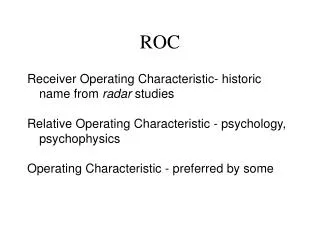
ROC Curves. ROC (Receiver Operating Characteristic) curve. ROC curves were developed in the 1950's as a by-product of research into making sense of radio signals contaminated by noise. More recently it's become clear that they are remarkably useful in decision-making.

E N D
ROC (Receiver Operating Characteristic) curve • ROC curves were developed in the 1950's as a by-product of research into making sense of radio signals contaminated by noise. More recently it's become clear that they are remarkably useful in decision-making. • They are a performance graphing method. • True positive and False positive fractions are plotted as we move the dividing threshold. They look like:
True positives and False positives True positive rate is TP = P correctly classified / P False positive rate is FP = N incorrectly classified as P / N
ROC Space • ROC graphs are two-dimensional graphs in which TP rate is plotted on the Y axis and FP rate is plotted on the X axis. • An ROC graph depicts relative trade-offs between benefits (true positives) and costs (false positives). • Figure shows an ROC graph with five classifiers labeled A through E. • A discrete classier is one that outputs only a class label. • Each discrete classier produces an (fp rate, tp rate) pair corresponding to a single point in ROC space. • Classifiers in figure are all discrete classifiers.
Several Points in ROC Space • Lower left point (0, 0) represents the strategy of never issuing a positive classification; • such a classier commits no false positive errors but also gains no true positives. • Upper right corner (1, 1) represents the opposite strategy, of unconditionally issuing positive classifications. • Point (0, 1) represents perfect classification. • D's performance is perfect as shown. • Informally, one point in ROC space is better than another if it is to the northwest of the first • tp rate is higher, fp rate is lower, or both.
“Conservative” vs. “Liberal” • Classifiers appearing on the left hand-side of an ROC graph, near the X axis, may be thought of as “conservative” • they make positive classifications only with strong evidence so they make few false positive errors, • but they often have low true positive rates as well. • Classifiers on the upper right-hand side of an ROC graph may be thought of as “liberal” • they make positive classifications with weak evidence so they classify nearly all positives correctly, • but they often have high false positive rates. • In figure, A is more conservative than B.
Random Performance • The diagonal line y = x represents the strategy of randomly guessing a class. • For example, if a classier randomly says “Positive” half the time (regardless of the instance provided), it can be expected to get half the positives and half the negatives correct; • this yields the point (0.5; 0.5) in ROC space. • If it randomly say “Positive” 90% of the time (regardless of the instance provided), it can be expected to: • get 90% of the positives correct, but • its false positive rate will increase to 90% as well, yielding (0.9; 0.9) in ROC space. • A random classier will produce a ROC point that "slides" back and forth on the diagonal based on the frequency with which it guesses the positive class. C's performance is virtually random. At (0.7; 0.7), C is guessing the positive class 70% of the time.
Upper and Lower Triangular Areas • To get away from the diagonal into the upper triangular region, the classifier must exploit some information in the data. • Any classifier that appears in the lower right triangle performs worse than random guessing. • This triangle is therefore usually empty in ROC graphs. • If we negate a classifier that is, reverse its classification decisions on every instance, then: • its true positive classifications become false negative mistakes, and • its false positives become true negatives. • A classifier below the diagonal may be said to have useful information, but it is applying the information incorrectly
Curves in ROC space • Many classifiers, such as decision trees or rule sets, are designed to produce only a class decision, i.e., a Y or N on each instance. • When such a discrete classier is applied to a test set, it yields a single confusion matrix, which in turn corresponds to one ROC point. • Thus, a discrete classifier produces only a single point in ROC space. • Some classifiers, such as a Naive Bayes classifier, yield an instance probability or score. • Such a ranking or scoring classier can be used with a threshold to produce a discrete (binary) classier: • if the classier output is above the threshold, the classier produces a Y, • else a N. • Each threshold value produces a different point in ROC space (corresponding to a different confusion matrix). • Conceptually, we may imagine varying a threshold from –infinity to + infinity and tracing a curve through ROC space.
Algorithm • Exploit monotonicity of thresholded classifications: • Any instance that is classified positive with respect to a given threshold will be classified positive for all lower thresholds as well. • Therefore, we can simply: • sort the test instances decreasing by their scores and • move down the list, processing one instance at a time and • update TP and FP as we go. • In this way, an ROC graph can be created from a linear scan.
Example A threshold of +inf produces the point (0; 0). As we lower the threshold to 0.9 the first positive instance is classified positive, yielding (0;0.1). As the threshold is further reduced, the curve climbs up and to the right, ending up at (1;1) with a threshold of 0.1. Lowering this threshold corresponds to moving from the “conservative” to the “liberal” areas of the graph.
Observations – Accuracy • The ROC point at (0.1, 0.5) produces its highest accuracy (70%). • Note that the classifier's best accuracy occurs at a threshold of .54, rather than at .5 as we might expect with a balanced class distribution.
Creating Scoring Classifiers • Many discrete classier models may easily be converted to scoring classifiers by “looking inside” them at the instance statistics they keep. • For example, a decision tree determines a class label of a leaf node from the proportion of instances at the node; the class decision is simply the most prevalent class. • These class proportions may serve as a score.
Area under an ROC Curve • AUC has an important statistical property: The AUC of a classifier is equivalent to the probability that the classier will rank a randomly chosen positive instance higher than a randomly chosen negative instance. • Often used to compare classifiers: • The bigger AUC the better • AUC can be computed by a slight modification to the algorithm for constructing ROC curves.
Convex Hull • The shaded area is called the convex hull of the two curves. • You should operate always at a point that lies on the upper boundary of the convex hull. • What about some point in the middle where neither A nor B lies on the convex hull? • Answer: “Randomly” combine A and B If you aim to cover just 40% of the true positives you should choose method A, which gives a false positive rate of 5%. If you aim to cover 80% of the true positives you should choose method B, which gives a false positive rate of 60% as compared with A’s 80%. If you aim to cover 60% of the true positives then you should combine A and B.
Combining classifiers • Example (CoIL Symposium Challenge 2000): • There is a set of 4000 clients to whom we wish to market a new insurance policy. • Our budget dictates that we can afford to market to only 800 of them, so we want to select the 800 who are most likely to respond to the offer. • The expected class prior of responders is 6%, so within the population of 4000 we expect to have 240 responders (positives) and 3760 non-responders (negatives).
Combining classifiers • Assume we have generated two classifiers, A and B, which score clients by the probability they will buy the policy. • In ROC space, • A’s best point lies at (.1, .2) and • B’s best point lies at (.25, .6) • We want to market to exactly 800 people so our solution constraint is: • fp rate * 3760 + tp rate * 240 = 800 • If we use A, we expect: • .1 * 3760 + .2*240 = 424 candidates, which is too few. • If we use B we expect: • .25*3760 + .6*240 = 1084 candidates, which is too many. • We want a classifier between A and B.
Combining classifiers • The solution constraint is shown as a dashed line. • It intersects the line between A and B at C, • approximately (.18, .42) • A classifier at point C would give the performance we desire and we can achieve it using linear interpolation. • Calculate k as the proportional distance that C lies on the line between A and B: k = (.18-.1) / (.25 – .1) 0.53 • Therefore, if we sample B's decisions at a rate of .53 and A's decisions at a rate of 1-.53=.47 we should attain C's performance. • In practice this fractional sampling can be done as follows: • For each instance (person), generate a random number between zero and one. • If the random number is greater than k, apply classier A to the instance and report its decision, else pass the instance to B.
The Inadequacy of Accuracy • As the class distribution becomes more skewed, evaluation based on accuracy breaks down. • Consider a domain where the classes appear in a 999:1 ratio. • A simple rule, which classifies as the maximum likelihood class, gives a 99.9% accuracy. • Presumably this is not satisfactory if a nontrivial solution is sought. • Evaluation by classification accuracy also tacitly assumes equal error costs---that a false positive error is equivalent to a false negative error. • In the real world this is rarely the case, because classifications lead to actions which have consequences, sometimes grave.
Iso-Performance lines • Let c(Y,n) be the cost of a false positive error. • Let c(N,p) be the cost of a false negative error. • Let p(p) be the prior probability of a positive example • p(n) = 1- p(p) is the prior probability of a negative example • The expected cost of a classification by the classifier represented by a point (TP, FP) in ROC space is: p(p) * (1-TP) * c(N,p) + p(n) * FP * c(Y,n) • Therefore, two points (TP1,FP1) and (TP2,FP2) have the same performance if (TP2 – TP1) / (FP2-FP1) = p(n)c(Y,n) / p(p)c(N,p)
Iso-Performance lines • The equation defines the slope of an isoperformance line, i.e., all classifiers corresponding to points on the line have the same expected cost. • Each set of class and cost distributions defines a family of isoperformance lines. • Lines “more northwest”---having a larger TP intercept---are better because they correspond to classifiers with lower expected cost. Lines and show the optimal classifier under different sets of conditions.
Cost based classification • Let {p,n} be the positive and negative instance classes. • Let {Y,N} be the classifications produced by a classifier. • Let c(Y,n) be the cost of a false positive error. • Let c(N,p) be the cost of a false negative error. • For an instance E, • the classifier computes p(p|E) andp(n|E)=1- p(p|E) and • the decision to emit a positive classification is [1-p(p|E)]*c(Y,n) < p(p|E) * c(N,p)