Download
1 / 47
470 likes | 629 Views
Predicting the Next Sunspot Cycle. Dr. David H. Hathaway NASA/NSSTC 2007 February 16. Outline. Significance of space weather Predicting the current sunspot cycle Predicting the next sunspot cycle with “precursors” Predicting the next sunspot cycle with dynamo models Conclusions.

E N D
Predicting the Next Sunspot Cycle Dr. David H. Hathaway NASA/NSSTC 2007 February 16
Outline • Significance of space weather • Predicting the current sunspot cycle • Predicting the next sunspot cycle with “precursors” • Predicting the next sunspot cycle with dynamo models • Conclusions
Space Weather Space weather refers to conditions on the Sun and in the space environment that can influence the performance and reliability of space-borne and ground-based technological systems, and can endanger human life or health. • Sources of Space Weather • Photons (X-rays, EUV) • Energetic Particles (Protons) • Magnetized Plasma
Example: The Bastille Day Event The flare, seen in EUV, emits energetic photons and accelerates particles. The coronal mass ejection, also accelerates particles and ejects magnetized plasma from the Sun. The energetic par-ticles shower the imaging instruments on SOHO minutes later.
Effects of Solar Activity:On Human Space Flight Shuttle missions and EVAs require particular attention. The Space Radiation Analysis Group (SRAG) reports to Mission Control when: K-index > 6, X-Ray Flux > M5, Protons at >100 MeV > 50. ISS: 50 pfu at > 100 MeV - shutdown the robotic arm 100 pfu at > 100 MeV - alert Mission Control. The Flight Team will start to evaluate a plan to shutdown equipment to prevent damage. 200 pfu at > 100 MeV - plan is implemented
Effects of Solar Activity: On Satellites Radiation (protons, electrons, alpha particles) from solar flares and coronal mass ejections can damage electronics on satellites. Heating of the Earth’s upper atmosphere increases satellite drag. • 1991 GOES • 1995 Deutsche Telekom • 1996 Telesat Canada • 1997 Telstar 401 • 2000/07/14 ASCA • 2003 Mars Odyssey • 4500 spacecraft anomalies over last 25 years
Effects of Solar Activity: On Power Grids Solar disturbances shake the Earth’s magnetic field. This sets up huge electrical currents in power lines and pipe lines. The solar storm of March 13th 1989 fried a $10M transformer in NJ. The same storm interrupted power to the province of Quebec for 6 days.
HF Communication only Effects of Solar Activity: On Airline Operations • Polar flights departing from North America use VHF (30-300 MHz) comm or Satcom with Canadian ATCs and Arctic Radio. • Flights rely on HF (3 – 30 MHz) communication inside the 82 degree circle. • Growth: Airlines operating China-US routes goes from 4 to 6 and then number of weekly flights goes from 54 to 249 over the next 6-years.
Effects of Solar Activity: On Climate? Yearly Sunspot Numbers and Reconstructed Northern Hemis-phere Temperature (Mann, Bradley & Hughes Nature 392, 779-787, 1998) smoothed with an 11-year FWHM tapered Gaussian and trimmed to valid smoothed data. The correlation coefficient from the overlapping period is 0.78 but the physical mechanism linking the two is unknown.
The “11-year” Sunspot Cycle The sunspot cycle was discovered by Heinrich Schwabe in 1844 from 18-years of personal observations. The cycle periods are normally distributed about 131 months with a variance of 14 months.
Sunspot Cycle Amplitude Variation Sunspot cycles vary widely in amplitude with occasional periods of inactivity like the Maunder Minimum (1645-1715). The cycle amplitudes have varied from a low of 45 to a high of 190 (in yearly averages of the daily sunspot number) since 1745.
Sunspot Area 10.7cm Radio Flux GOES X-Ray Flares Total Irradiance Geomagnetic aa index Climax Cosmic-Ray Flux Sunspot Number and Solar Activity Sunspot number is well correlated with other indicators of solar activity. The long record of sunspot numbers helps to better characterize the solar cycle. Predicting the sunspot number also provides an estimate of these other source of solar activity.
Sunspot Cycle Shape Waldmeier (1935, 1939) noted that the sunspot cycles were asymmetric with shorter rise times and longer decay times. Furthermore, small cycles take longer to rise to maximum than do large cycles. Hathaway, Wilson, & Reichmann (1994) constructed a function of two parameters (starting time and amplitude) which reproduces this behavior. The Waldmeier Effect The HWR Function
Two Parameter (Per Cycle) Fit The two-parameter function fits the sunspot cycle behavior well (with the possible exception of two cycles prior to 1854 when the data was questionable).
Parameters Determined Early Both the amplitude and the starting time are well determined 2-3 years after the start of a cycle. Recall that maximum occurs 4-6 years after the start of a cycle.
Prediction at month 30 Prediction for the Current Cycle Reliable predictions for the level of solar activity in the current cycle become available about 30-months after minimum (at about the inflection point on the rise).
Precursor Techniques Techniques other than curve-fitting or auto-regression are needed to predict cycle amplitudes at times near or before sunspot cycle minimum. 1) Use the average cycle. 2) Use trends or periodicities in cycle amplitudes. 3) Use information from cycle statistics. 4) Use information from other cycle indicators, specifically the geomagnetic indices and polar fields.
Secular Trend Since Maunder Minimum The sunspot cycle amplitude shows a significant secular increase since the Maunder Minimum. The standard deviation about an average cycle amplitude is 36, the standard deviation about the secular trend reduces this to 24.
Multi-Cycle Periodicities? After removing the secular trend, there is little evidence for any significant periodic behavior with periods of 2-cycles (Gnevyshev-Ohl) or 3-cycles (Ahluwalia) There is some evidence for periodic behavior with a period of about 9-cycles (Gleissberg).
Amplitude-Period Effect The amplitude of a cycle is anti-correlated to the period of the previous cycle. Large cycles follow short cycles.
Amplitude-Minimum Effect The amplitude of a cycle is correlated with the size of the minimum that precedes the cycle.
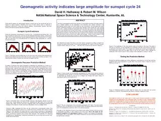
Geomagnetic Precursors Geomagnetic activity around the time of minimum seems to give an indication of the size of the next maximum. Ohl (1966) found that the minimum in the geomagnetic index aa could predict the next maximum.
Testing Precursor Techniques Hathaway, Wilson, & Reichmann (1999) 1) Back up in time to the beginning of each of the last five cycles. 2) Using only information from earlier times, recalibrate each technique and apply the results to that cycle. 3) Compare the predictions with the actual numbers. Prediction Method Errors (Prediction-Observed)
Feynman’s Method Hathaway & Wilson (2006) Joan Feynman (1984) noted that the minimum level of geomagnetic activity increased linearly with the sunspot number. She identified this with a solar cycle related component of geomagnetic activity. Subtracting that level leaves behind an “Interplanetary” component that mimics the sunspot number but leads it by several years!
Feynman Method Predictionfor Cycle 24 We find a peak in the “Interplanetary” component in late 2003 that gives a predicted amplitude for cycle 24 of 160±30.
The Sun’s Magnetic Cycle • The high conductivity of the fluid within the Sun makes the magnetic field and the fluid flow together (frozen in field lines). • The high pressures found inside the Sun insures that the fluid flow controls the magnetic field (except in the centers of sunspots).
The Babcock-Leighton Dynamo • Babcock (1961) and Leighton (1969) proposed a magnetic dynamo based on two processes identified by Parker (1955). • Stretching by latitudinal differential rotation • (the Omega Effect) • Lifting and twisting by buoyancy • (the Alpha Effect)
Polar Field Strength Predictions Schatten et al (1978, with many papers following) have used the strength of the polar fields near the time of minimum to predict the amplitude of the following maximum. Accuracy has been similar to that of the geomagnetic precursors. Prediction Errors One problem with this technique is that we have polar field data for only the last three cycles. A second problem is the lack of any guidance on when the polar measurements should be taken. Svalgaard, Cliver, Kamide (2005) find that the polar fields now are about half what they were at previous minima and predict an amplitude for cycle 24 of 75 ± 8.
Dynamos with Meridional Flow Recent Dynamo models incorporate a deep meridional flow to transport magnetic flux toward the equator at the base of the convection zone. These models explain the equatorward drift of activity, the poleward drift of weak magnetic elements on the surface, the length of the cycle from the speed of the flow, and give a relationship between polar fields at minimum and the amplitude of future cycles. Dikpati and Charbonneau, ApJ 518, 508-520, 1999
Latitude Drift of Sunspot Zones We examined the latitude drift of the sunspot zones by first separating the cycles where they overlap at minimum. We then calculated the centroid position of the daily sunspot area averaged over solar rotations for each hemisphere. [Hathaway, Nandy, Wilson, & Reichmann, ApJ 589. 665-670 2003 & ApJ 602, 543-543 2004]
Drift Rate vs. Latitude The drift rate in each hemisphere and for each cycle (with one exception) slows as the activity approaches the equator. This behavior is expected from dynamo models with deep meridional flow.
Drift Rate – Period Anti-correlation The sunspot cycle period is anti-correlated with the drift velocity at cycle maximum. The faster the drift rate the shorter the period. This is also expected from dynamo models with deep meridional flow. R=-0.5 95% Significant
Drift Rate – Amplitude Correlations We find that the drift velocity at cycle maximum is correlated to the amplitude of the second following (N+2) cycle maximum. The correlation is much weaker for the (N+1) or (N+3) maximum. R=0.7 99% Significant
Cycle 24 Amplitude Prediction Based on the fast drift rates at the maximum of the last (22nd) cycle (red oval – northern hemisphere, yellow oval – southern hemisphere) we predict an amplitude of 145±30 for cycle 24.
The Dynamo Prediction Dikpati, de Toma & Gilman (2006) have fed sunspot areas and positions into their numerical model for the Sun’s dynamo and reproduced the amplitudes of the last eight cycles with unprecedented accuracy (RMS error < 10). Cycle 24 Prediction ~ 165 ± 15
Possible Problems • They used our data – which was 20% high for cycle 20. • Their prediction for the actual size of cycle 20 was good but later cycles were also predicted accurately in spite of the error in the input data. • They kept the meridional flow speed constant. • They allow it to change in cycle 23 and find a 10% change in the prediction. Similar variations in meridional flow speed should have occurred in the past. • The latitudes at which they introduced the sunspot magnetic fields were not representative of the actual latitudes. • They had sunspots start the cycle at 35° and drift linearly to 5° over exactly 11 years. A far better representation is a parabolic trajectory from 25° down to 8°.
Recent Developments The Dikpati et al. (2006) prediction, based firmly in dynamo theory, is the leading contender. Consequently, it is taking a lot of heat. • Tobais, Hughes, & Weiss (2006) corresponded in Nature with a letter titled “Unpredictable Sun leaves researchers in the dark” and claimed “parameterization of many poorly understood effects … have no detailed predictive power” • Cameron & Schussler (2007) have a paper in press in ApJ showing similar predictive power in a simple 1D flux transport model for the surface magnetic field – provided the parameters are tuned to those of Dikpati et al. (2006). The predictive power virtually disappears when detailed sunspot information is used. • Choudhuri, Chatterjee, & Jaing have submitted a paper to Phys. Rev. Lett. in which they feed the observed polar fields from the last three cycles into their 2D code, find good agreement with the sunspot numbers and predict a small cycle 24.
The Question of Timing Predicting the start of the next cycle is just as difficult as predicting its amplitude. Statistics such as the number of spotless days and the level of activity itself provide some guidance but with significant scatter. Statistics also tell us that big cycles usually start early while small cycles start late. The Dikpati et al. dynamo model tells us that the slow meridional flow during the current cycle should delay the start of the next cycle. The best indicator for the start of a new cycle is the start of a new cycle – the appearance of reversed polarity sunspots at latitudes well above 20°.
“Backwards” Sunspots Southern hemisphere sunspots for cycle 23 had positive polarities to the left and negative polarities to the right. On July 30th 2006 a magnetic dipole erupted in the south with “backwards” polarity expected for cycle 24 sunspots. A small sunspot formed for just a couple hours.
“Backwards” Sunspots On August 21th 2006 another “backwards” sunspot rotated onto the disk and this time remained visible for its full disk passage. Again, however, the low latitude of this spot (8° South) makes its identification as a Cycle 24 sunspot unlikely.
New Cycle Sunspot Remains? On November 27th 2006 a reversed polarity region, without any sunspot, rotated into view from the backside of the Sun. Was this the remains of the first, but unobserved, sunspot of the new cycle?
Conclusions • Explicit modeling of the cycles since 1880 using sunspot areas as input accurately predicts the amplitudes of the last eight cycles and predicts a large amplitude for the next cycle. • The Geomagnetic precursors, the secular trend in cycle amplitudes, and the drift rate of the active latitudes all indicate a much larger than average cycle 24. • Polar field strength indicates a very small amplitude cycle 24. • Reconciling these differences requires a better understanding, as well as independent confirmation, of the dynamo models.
Long-Range Prediction Based on the fast drift rates at the maximum of the last (22nd) cycle (red oval – northern hemisphere, yellow oval – southern hemisphere) we predict a large amplitude for the next cycle (24th). Slow drift rates during cycle 23 indicate a very small cycle 25.