Download
1 / 74
740 likes | 917 Views
Consistent Linear-Elastic Transformations for Image Matching. Gary E. Christensen Department of Electrical & Computer Engineering The University of Iowa. This work was supported by NIH grant NS35368 and a grant from the Whitaker Foundation. Introduction. Uses of image registration

E N D
Consistent Linear-Elastic Transformations for Image Matching Gary E. Christensen Department of Electrical & Computer Engineering The University of Iowa This work was supported by NIH grant NS35368 and a grant from the Whitaker Foundation.
Introduction • Uses of image registration • image segmentation/deformable atlas • characterization of normal vs. abnormal shape/variation • multi-modality fusion • functional brain mapping/removing shape variation • surgical planning and evaluation • image guided surgery • template constrained reconstruction • Image registration methods • landmark, contour, surface, volume
Introduction • Landmarks specify correspondence. • Transformation interpolated between landmarks. • Ideally, forward and reverse transforms are inverses of each other.
Introduction • Limitations • Landmark • manual identification, low-dimensional • Contour • manual/semi-automatic, correspondence ambiguity • Surface • semi-automatic/automatic, correspondence ambiguity • Volume • automatic, correspondence ambiguity
Introduction • Woods et al., Automated Image Registration: II. Intersubject Validation of Linear and Nonlinear Models, Journal of Computer Assisted Tomography, 22(1), 1998 • Pairwise consistency • Compute all pairwise registrations of a population using the affine transformation model. • Average the transformation from A to B with all the transformations from A to X to B. • Replace the original transformation from A to B with average transformation. Repeat for all until convergence.
Introduction • Woods et al., Automated Image Registration: II. Intersubject Validation of Linear and Nonlinear Models, Journal of Computer Assisted Tomography, 22(1), 1998 • Limitations • Does not apply for a population of two data sets. • There is no guarantee that the generated set of consistent transformations are valid. • ex. A poorly registered pair of images can adversely effect all of the pairwise transformations.
Introduction • Consistent Transformation Estimation • Jointly estimate the forward and reverse transformation between two image volumes • Constrain the forward and reverse transformations to be inverses • Constrain the transformations to preserve topology
Problem Statement • Jointly estimate the transformations h and g such that h maps T to S and g maps S to T subject to the constraint that h = g-1
Transformation Properties • From a biological standpoint, it is desirable that image registration algorithms produce transformations with the properties: • The transformation from image A to B is unique, i.e., the forward hab and reverse hba transformations are inverses of one another. • The transformations have the transitive property, i.e., hab(hbc(x)) = hac(x). • Most image registration algorithms do not produce transformations with these properties.
Sources of Error:Inverse Consistency Error (EICC) y=g(x) x’ y x x’ =h(y) Inverse Consistency Error = ||x-x’|| where x’=h(g(x))
2D Landmark Experiment Forward Reverse • Compare thin-plate spline algorithms • Unidirectional vs. consistent registration* • *Consistent Landmark Registration: 2000 iterations, X harmonics = 50, Y harmonics = 50
5.0 Consistent TPS 0.00 Inverse Consistency Error(Cyclic Boundary Conditions) A—B—A B—A—B A—B—A 5.0 TPS 0.00
0.01 Consistent TPS 0.00 Inverse Consistency Error(Cyclic Boundary Conditions) A—B—A B—A—B A—B—A 5.0 TPS 0.00
D D B B C C A A Inverse Consistency Error(Cyclic Boundary Conditions) A—B—A B—A—B 5.0 TPS 0.00 0.01 Consistent TPS 0.00
Notation • Image volumes: • T(x) = Template S(x) = Target • Coordinate system: • Transformations:
Symmetric Similarity Function • Jointly estimate transformations from T to S and from S to T • Minimize cost w.r.t. h and g • Works with any similarity function • mutual information
Inverse Transformation Consistency • Symmetric similarity functions do not guarantee g and h are inverses of each other. • Impose constraint that g and h are inverses.
Diffeomorphic Transformations h: • Onto • Globally One-to-One • Continuous • Compact sets are mapped to compact sets • Connected sets are mapped to connected sets • A composition of continuous transformations is continuous • Differentiable
Diffeomorphic Constraint • The inverse consistency constraint only guarantees h and g are diffeomorphic transformations when • To constrain h and g to be diffeomorphic, we use continuum mechanical models • linear elasticity • viscous fluid
Diffeomorphic Constraint • Linear Elasticity
1D Example • Complex exponentials are eigenfunctions of constant coefficient difference equations
Transformation Parameterization • Displacement fields (cyclic boundary conditions) • coefficients • (3x1) complex-valued vectors • complex conjugate symmetry
Diffeomorphic Constraint • Combining • Gives
Diffeomorphic Constraint • Linear Elasticity constraint
Minimization Problem ^ • Find h and g that satisfy: ^ l and r are Lagrange multipliers
Consistent Landmark • Consistent Landmark Cost Minimization
Minimization Algorithm • Gradient descent is used to solve for new basis coefficients at each iteration. • Coarse to fine registration • Start algorithm with 0 and 1st harmonics. • Increase the number of harmonics by one after every N iterations. • The reverse basis coefficients are fixed while estimating the forward basis coefficients and visa versa.
Inverse Transformation Computation • Gradient Descent • Solution exists and is unique if h is a monotonic function of x • h is diffeomorphic => h is monotonic in x
3D CT Inverse Consistency Experiment • Use 3D CT data of infant heads • Transform data volume A to B, and vice versa • Traditional linear-elasticity model • Consistent linear-elasticity model • Combine the forward & reverse transformations • Compare the composite transformation to Identity
3D CT Inverse Consistency Experiment Error of composite mapping hab(hba(x)) using the linear elastic model without inverse consistency constraint. 1.2 Coronal Sagittal Axial -0.94 X-Dev. Y-Dev. Z-Dev. Mag. Dev.
3D CT Inverse Consistency Experiment Error of composite mapping hab(hba(x)) with inverse consistency constraint using the linear elastic model. 0.1 Coronal Sagittal Axial -0.1 X-Dev. Y-Dev. Z-Dev. Mag. Dev.
1.2 -0.94 0.1 -0.1 X-Dev. Y-Dev. Z-Dev. Mag. Dev. 3D CT Inverse Consistency Experiment Error of composite mapping hab(hba(x)) using the linear elastic model with & without inverse consistency constraint. Without inverse consistency With inverse consistency
3D CT Inverse Consistency Experiment Error of composite mapping hab(hba(x)) using the linear elastic model with and without inverse consistency constraint. FH-Frankfurt Horizontal Plane
Experiments • Eight experiments: • MRI1: no constraints • MRI2: linear elasticity • MRI3: inverse consistency • MRI4: lin. elast. and inv. consist. • CT1: no constraints • CT2: linear elasticity • CT3: inverse consistency • CT4: lin. elast. and inv. consist.
T S T(h) S(g) u1 u2 u3 w1 w2 w3 MRI4 Experiment Christensen, IPMI’99
MRI4 Experiment Christensen, IPMI’99
MRI4 Experiment Christensen, IPMI’99
MRI4 Experiment Christensen, IPMI’99
MRI4 Experiment Christensen, IPMI’99
Transformation Measurements ~ ~ Christensen, IPMI’99
T S T(h) S(g) u1 u2 u3 w1 w2 w3 CT4 Experiment Christensen, IPMI’99
CT4 Experiment Christensen, IPMI’99
CT4 Experiment Christensen, IPMI’99
CT4 Experiment Christensen, IPMI’99
CT4 Experiment Christensen, IPMI’99
Transformation Measurements ~ ~ Christensen, IPMI’99
Transformation Measurements ~ ~ Christensen, IPMI’99
Computational Costs • Computational efficiency was achieved by using FFTs. • Transforming one 643 voxel volume into another using 300 iterations takes approximately 25 minutes on a 180 MHz, R10000 processor. • Computational time can be reduced by • reducing the number of iterations • using a more efficient optimization algorithm such as conjugate gradient, etc.
Anatomical Variation • Goal is to quantify the average shape & variability of anatomical populations.
Literature • Joshi et al., Gaussian Random Fields on Sub-manifolds for Characterizing Brain Surfaces, XVth International Conference on Information Processing in Medical Imaging, eds. Duncan and Gindi, Poultney, VT, June,1997 • Miller et al., Statistical Methods in Computational Anatomy, Statistical Methods in Medical Research, vol. 6, 1997 • Woods et al., Automated Image Registration: II. Intersubject Validation of Linear and Nonlinear Models, Journal of Computer Assisted Tomography, 22(1), 1998