Image matching

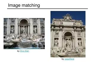
1. Image matching by Diva Sian by swashford TexPoint fonts used in EMF. Read the TexPoint manual before you delete this box.: AAAAAA

2. Harder case by Diva Sian by scgbt

3. Even harder case “How the Afghan Girl was Identified by Her Iris Patterns” Read the story

4. Harder still? NASA Mars Rover images

5. Answer below (look for tiny colored squares…) NASA Mars Rover images with SIFT feature matchesFigure by Noah Snavely

6. Features All is Vanity, by C. Allan Gilbert, 1873-1929 • Reading • M. Brown et al. Multi-Image Matching using Multi-Scale Oriented Patches, CVPR 2005

7. Image Matching

8. Image Matching

9. Invariant local features Find features that are invariant to transformations • geometric invariance: translation, rotation, scale • photometric invariance: brightness, exposure, … Feature Descriptors

10. Advantages of local features Locality • features are local, so robust to occlusion and clutter Distinctiveness: • can differentiate a large database of objects Quantity • hundreds or thousands in a single image Efficiency • real-time performance achievable

11. More motivation… Feature points are used for: • Image alignment (e.g., panoramas) • 3D reconstruction • Motion tracking • Object recognition • Indexing and database retrieval • Robot navigation • … many others

12. What makes a good feature? Snoop demo

13. Want uniqueness Look for image regions that are unusual • Lead to unambiguous matches in other images How to define “unusual”?

14. Local measures of uniqueness Suppose we only consider a small window of pixels • What defines whether a feature is a good or bad candidate? Slide adapted from Darya Frolova, Denis Simakov, Weizmann Institute.

15. Feature detection Local measure of feature uniqueness • How does the window change when you shift by a small amount? “corner”:significant change in all directions “flat” region:no change in all directions “edge”: no change along the edge direction Slide adapted from Darya Frolova, Denis Simakov, Weizmann Institute.

16. We want to be ______ Feature detection Define E(u,v) = amount of change when you shift the window by (u,v) E(u,v) is small for no shifts E(u,v) is small for all shifts E(u,v) is small for some shifts

17. Feature detection: the math • Consider shifting the window W by (u,v) • how do the pixels in W change? • compare each pixel before and after bySum of the Squared Differences (SSD) • this defines an SSD “error” E(u,v): W

18. Small motion assumption Taylor Series expansion of I: If the motion (u,v) is small, then first order approx is good Plugging this into the formula on the previous slide…

19. Feature detection: the math • Consider shifting the window W by (u,v) • how do the pixels in W change? • compare each pixel before and after bysumming up the squared differences • this defines an “error” of E(u,v): W

20. Feature detection: the math This can be rewritten: • For the example above • You can move the center of the green window to anywhere on the blue unit circle • Which directions will result in the largest and smallest E values? • We can find these directions by looking at the eigenvectors ofH

21. Quick eigenvalue/eigenvector review The eigenvectors of a matrix A are the vectors x that satisfy: The scalar λ is the eigenvalue corresponding to x • The eigenvalues are found by solving: • In our case, A = H is a 2x2 matrix, so we have • The solution: Once you know λ, you find x by solving

22. Feature detection: the math This can be rewritten: x- x+ • Eigenvalues and eigenvectors of H • Define shifts with the smallest and largest change (E value) • x+ = direction of largest increase in E. • λ+ = amount of increase in direction x+ • x- = direction of smallest increase in E. • λ- = amount of increase in direction x+

23. Feature detection Local measure of feature uniqueness • E(u,v) = amount of change when you shift the window by (u,v) E(u,v) is small for no shifts E(u,v) is small for all shifts E(u,v) is small for some shifts We want to be large = ?

24. Eigenvalues of H

25. Feature detection summary • Here’s what you do • Compute the gradient at each point in the image • Create the H matrix from the entries in the gradient • Compute the eigenvalues. • Find points with large response (λ- > threshold) • Choose those points where λ- is a local maximum as features

26. Feature detection summary • Here’s what you do • Compute the gradient at each point in the image • Create the H matrix from the entries in the gradient • Compute the eigenvalues. • Find points with large response (λ- > threshold) • Choose those points where λ- is a local maximum as features

27. The Harris operator • λ- is a variant of the “Harris operator” for feature detection • The trace is the sum of the diagonals, i.e., trace(H) = h11 + h22 • Very similar to λ- but less expensive (no square root) • Called the “Harris Corner Detector” or “Harris Operator” • Lots of other detectors, this is one of the most popular

28. The Harris operator Harris operator

29. Harris detector example

30. f value (red high, blue low)

31. Threshold (f > value)

32. Find local maxima of f

33. Harris features (in red)

34. Invariance Suppose you rotate the image by some angle • Will you still pick up the same features? What if you change the brightness? Scale?

35. Scale invariant detection Suppose you’re looking for corners Key idea: find scale that gives local maximum of f • f is a local maximum in both position and scale • Common definition of f: Laplacian(or difference between two Gaussian filtered images with different sigmas)

36. Feature descriptors We know how to detect good points Next question: How to match them? ?

37. Feature descriptors We know how to detect good points Next question: How to match them? Lots of possibilities (this is a popular research area) • Simple option: match square windows around the point • State of the art approach: SIFT • David Lowe, UBC http://www.cs.ubc.ca/~lowe/keypoints/ ?

38. Invariance Suppose we are comparing two images I1 and I2 • I2 may be a transformed version of I1 • What kinds of transformations are we likely to encounter in practice?

39. Invariance Suppose we are comparing two images I1 and I2 • I2 may be a transformed version of I1 • What kinds of transformations are we likely to encounter in practice? We’d like to find the same features regardless of the transformation • This is called transformational invariance • Most feature methods are designed to be invariant to • Translation, 2D rotation, scale • They can usually also handle • Limited 3D rotations (SIFT works up to about 60 degrees) • Limited affine transformations (some are fully affine invariant) • Limited illumination/contrast changes

40. How to achieve invariance Need both of the following: • Make sure your detector is invariant • Harris is invariant to translation and rotation • Scale is trickier • SIFT uses automatic scale selection (previous slides) • simpler approach is to detect features at many scales using a Gaussian pyramid (e.g., MOPS) and add them all to database 2. Design an invariant feature descriptor • A descriptor captures the information in a region around the detected feature point • The simplest descriptor: a square window of pixels • What’s this invariant to? • Let’s look at some better approaches…

41. Rotation invariance for feature descriptors Find dominant orientation of the image window • This is given by x+, the eigenvector of H corresponding to λ+ • λ+ is the larger eigenvalue • Rotate the window according to this angle Figure by Matthew Brown

42. Multiscale Oriented PatcheS descriptor Take 40x40 square window around detected feature • Scale to 1/5 size (using prefiltering) • Rotate to horizontal • Sample 8x8 square window centered at feature • Intensity normalize the window by subtracting the mean, dividing by the standard deviation in the window 8 pixels 40 pixels CSE 576: Computer Vision Adapted from slide by Matthew Brown

43. Detections at multiple scales

44. 2π 0 Scale Invariant Feature Transform • Basic idea: • Take 16x16 square window around detected feature • Compute edge orientation (angle of the gradient - 90°) for each pixel • Throw out weak edges (threshold gradient magnitude) • Create histogram of surviving edge orientations angle histogram Adapted from slide by David Lowe

45. SIFT descriptor • Full version • Divide the 16x16 window into a 4x4 grid of cells (2x2 case shown below) • Compute an orientation histogram for each cell • 16 cells * 8 orientations = 128 dimensional descriptor Adapted from slide by David Lowe

46. Properties of SIFT Extraordinarily robust matching technique • Can handle changes in viewpoint • Up to about 60 degree out of plane rotation • Can handle significant changes in illumination • Sometimes even day vs. night (below) • Fast and efficient—can run in real time • Lots of code available • http://people.csail.mit.edu/albert/ladypack/wiki/index.php/Known_implementations_of_SIFT

47. When does SIFT fail? Patches SIFT thought were the same but aren’t:

48. Feature matching Given a feature in I1, how to find the best match in I2? • Define distance function that compares two descriptors • Test all the features in I2, find the one with min distance

49. Feature distance How to define the difference between two features f1, f2? • Simple approach is SSD(f1, f2) • sum of square differences between entries of the two descriptors • can give good scores to very ambiguous (bad) matches f1 f2 I1 I2

50. Feature distance How to define the difference between two features f1, f2? • Better approach: ratio distance = SSD(f1, f2) / SSD(f1, f2’) • f2 is best SSD match to f1 in I2 • f2’ is 2nd best SSD match to f1 in I2 • gives large values (~1) for ambiguous matches f1 f2' f2 I1 I2