Download
1 / 59
590 likes | 670 Views
Diagnostics of the Galaxy Population in the Early Universe or Getting to the physically interesting quantities from observational ‘proxies’. Hans-Walter Rix March 24, 2009. Basic Goals of High-z Galaxy Studies. As a proxy for studying the typical evolutionary fates of individual galaxies,

E N D
Diagnostics of the Galaxy Population in the Early UniverseorGetting to the physically interesting quantities from observational ‘proxies’ Hans-Walter Rix March 24, 2009
Basic Goals of High-z Galaxy Studies As a proxy for studying the typical evolutionary fatesof individual galaxies, one needs to study the evolution of the galaxy population properties as a function of cosmic epoch. • At what epoch (redshift) was star-formation most vigorous? • When did the first ‘massive’ galaxies appear? • Need model comparison to go from observable population evolutiontoobject evolution.
Questions that can be answered by direct observations • Frequency of galaxies as function of • Epoch (Redshift) • Stellar Mass / Luminosity (Halo Mass?) • Spectral Energy Distribution (SED, color age) • Structure (size, bulge-to-disk) • Gas content (hot, cold) • What is the incidence of “special phases”? • (major) mergers; QSO-phases • How are these properties related to the larger “environment”?
Part I: Identifying High-z Galaxies Or To compare galaxy samples at different epochs, you need to know how you selected them
Issues in Sampling the high-z Galaxy Population • “Consistent” selection of galaxy samples becomes increasingly difficult as the redshift range expands. • K-correction (Fl,observed Fl,emitted) • (1+z)4 surface brightness dimming • Multi-variate distribution requires very large samples • Clustering of objects requires large-ish areas.
Search Strategies for High-z Galaxies • Size: 0.1” – 1” (almost independent of redshift) • Proxies for star-formation rate • UV, mid-IR and bolometric energy from young, massive stars • Proxies for stellar/halo mass? • “Foregrounds”, those pesty z~0.7 galaxies • Atmospheric windows and available technology
Single age pops. For a galaxy of given stellar mass, the SED depends drastically on- age of the stars-fraction of light absorbed by dust Devriend et al 2000
Practicalities of observing(high-redshift) galaxies SED of an ageing stellar population of solar metalicity with dust
.........................opt..NIR.................radio window....... 0.1nm 1 10 100 1mm 10 100 1cm 10 1m 10 100m wavelength Ground-based vs. space-based? NB: in addition to transmissivity, the emissivity of the Earth’s atmosphere is a big problem: sky at 2mm is 10,000 brighter than at 0.5mm Some sub-mm windows from good sites
XMM Chandra 2000 + HST 1991-2010 JWST 2014- Spitzer, Herschel 2004/2008 + Keck, VLT,LBT 1995-2025 ALMA, IRAM Observatories to Study Galaxies at Different l(here: a star-bursting galaxy with accreting black hole, and cold gas reservoir) X-rays, g-rays
“Foreground (z<2) Galaxies”when looking at a flux-limited sample NB: IAB=25 1 photon/year/cm2/A From: LeFevre, Vettolani et al 2003 “Brute force” spectroscopy is inefficient for z>2!
Star-Formation Rate Proxies • SFR Power and ionizing photons from hot, massive, short-lived stars. • UV flux and thermal-IR are the best and most practical proxies, but are inaccessible from the ground for z<1-2 • The peak of dust emission 100-300mm are almost inaccessible with current technology
Selecting Galaxies by their Rest-Frame UV Properties • Until mid-1990s only a handful of high-z galaxies were known (radio galaxies) • Breakthrough from the combination of color-selection and Keck spectroscopy (C. Steidel and collaborators, 1996 ff.) • “Break” arises from absorption of l<912A radiation through the intervening ISM and IGM
Ly-break Selection • Current sensitivity: >5 MSun/yr at z~3 (as inferred from UV-flux) • Very dusty galaxies or those with low-SFR will not be found. • Choice of filters sets redshift range • Z>2.2 from the ground • Ly-limit break at z~2 La break at z>4.5 • By now: > 2000 spectroscopically confirmed
Example of recent deep searches SUBARU Deep field
Typical SFRs in Ly-break Galaxies(from Pettini, Shapley et al 2003)
Selecting High-z Galaxies by their Emission Lines • UV photons in star-forming galaxies will excite Ly-a line • High contrast easier detection? From Shapley et al 2003
UV Continuum vs Ly-a Line Strongest Ly a emitters have • Bluest (=least reddened) stellar continua • Lowest warm-gas absorption gas/dust covering fraction and outflow structure determine line to continuum ratio Shapley et al 2003
Selecting Galaxies by their Rest-Frame Optical Emission • Selection less sensitive to high present star formation rate. • Still: populations fade in the rest-frame optical and IR, as populations age! • Less sensitive to dust extinction. • More differential comparison to lower-z population. • Note that lselection ~ (1+z) x 0.5mm ~ 2mm at z~3 deep (near-)infrared imaging
Example: FaintInfra-Red-Extragalactic-Survey HDF-south 100 hours in JHK MS1054: 6xlarger area 25 hours in JHK per pointing Franx, Rudnick, Labbe, Rix, Trujillo, Moorwood, et al. 2001-2004
Not a Ly-break!! Just a red SED
Photometric Redshift Estimation • Fit sequence of model population spectra to flux data points (=VERY low resolution spectrum) • Find best combination(s!) of SED and z • Use spectroscopic redshifts to check sub-samples
For robust photo-redshifts one needs at least one strong spectral break, either • Ly-break (912A - 1216A) or • “4000A”-break (Balmer break; H&K break) • broad spectral coverage, e.g. 0.3mm to 2.2mm
Data from the Spitzer satellite (3.5-8mm) help enormously in determining the SED of galaxies at z>2 stellar M/L, age etc.. (Wuyts, Franx, Rix et al 07)
Selecting Galaxies by their Thermal IR (sub-mm) Emission (from the ground)Smail et al, Ivison et al, Barger et al. 1998-2002 • Observations currently feasible only on the long-wavelength tail of the thermal dust emission • Sub-mm K-correction very favourable!! • Spatial resolution (single-dish) is low 5”-10” redshift Range of sub-mm observations
HDF at 850mm SCUBA array on the JCMT
The current generation of ‚machines‘ to study high-redshift galaxies Part II: Studying their Physical Properties Star Formation Rate Mass Gas Content Chemical Abundances
Estimating Star Formation Rates • Step 1: Verify that UV continuum is from stars and thermal-IR is powered by such stars (no AGN) • Step 2: assume IMF + SFR bolometric luminosity • Step 3: bolometric luminosity + dust content SED • Step 4: Scale SED to observations SFR (obs!)
Bolometric Luminosities from UV?in star-forming galaxies, most UV photons are absorbed by dustso … how do you use UV radiation to estimate the SFR? • Idea: extinction (=?absorption) is reflected in the UV continuum slope • L bol,dust = 1.66 L1600A ( 10 0.4(4.4+2b) -1) with ll~lb (Meuer, Heckman and Calzetti 1999)
How well does this work? Direct observations Based on this slope… ..they predict this..
Star-Formation Rates at high-redshift from the heated-dust emission Lbol up to 1013LSun SFRs to a few 1000 MSun/yr SED of a typical SCUBA source: IR emission completely dominates bolometric luminosity (from Ivison et al 2000)
Nature of SCUBA Sources: Star-burst or AGN? • Sub-mm data only demonstrate that dust is heated with enormous power • Check for AGN signatures: • Emission line diagnostics • X-ray emission? • Majority of them are star-bursts
Estimating (Cold) Gas Masses • True reservoir for star-formation • HI and H2 (currently) not detectable • Thermal dust emission ? Dust mass ?? Gas Mass • CO gas now detectable!! at mm wavelengths Plateau de Bure, F
Examples of extremely gas rich galaxies at z~2-3Neri et al 2003 (Plateau de Bure) M(H2) = a x L CO(1-2) with a = 0.8MSun(K km/s pc2)-1 for local ULIRGS M(gas) ~ 1-2 x 10¹⁰ MSun Rough estimates of Mdyn is only twice that!!
CO Gas at z~6.42:QSO host has vast gas reservoir Walter et al 2002
Estimating Stellar Masses • Kinematics/dynamics z>2 currently very hard • Spatial resolution • Ionized gas not (only) subject to gravity • Molecular gas only in very gas rich/rare(?) galaxies • Stellar SED to estimate M/L • Need (good) data beyond lrest ~ 4000 • Clustering (of galaxies) • vs clustering of halos in simulations
Dynamical Masses from COCase Study:SMMJ02399 (z=2.8)Genzel et al. 2003 Continuum/Dust emission Vrot = 420km/s! >3x10¹¹Msun within 6kpc
Ha Kinematics of high-redshift galaxies • N. Foerster Schreiber et al 2006 (SINFONI @ VLT) • When velocity fields are regular: Masses within optical radius comparable to SED-based stellar masses • Irregular velocity fields common mergers? Flux Velocity Dispersion Ha at z~2
Stellar Masses from SEDs • Age makes populations redder • Metallicity makes populations redder • Dust makes populations redder Degeneracies abound! But:all effects that make redder also increase the M/L in a similar fashion • good correlation SED vs M/L ! (Bell and de Jong 2001)
Estimating Chemical Abundances • Cosmic star-formation history implies progressive enrichment of • ISM • Stars that form from it • ‘Metals’ (=stellar nucleosynthesis products) are the ‘garbage’ of successive stellar population
Estimating ISM Abundancesin Galaxies at z>2 Erb et al 2007 @given M*, Fe/H used to be (at z=2) 2-3x lower
Estimating Stellar Metalicities(from the photospheres of stars)Mehlert et al 2002 FORS Deep Field • Typical stellar metallicities at z~2 are 1/3 as high as at z~0
“Cosmological Backgrounds” • Powerful constraint on the epoch-integrated, distance-weighted spectrum emitted by all sources From N. Wright
Summary • Z>2 Galaxies are being sampled by • UV continuum (many 1000) • Optical continuum (~1000) • Thermal-IR continuum (~100) “beasts” only • Ly-a emission (~100) strong bias in most techniques towards finding them during high star-formation phases z~6.5 current practical limit for samples • SFR estimates • from thermal-IR: robust, but tedious? (Spitzer+Herschel,ALMA) • Practical from the UV, but UV is usually strongly extincted!! • Mass estimates • CO dynamics: good, but large samples not yet feasible • From stellar SEDs: need very good IR data (lrest>4000A)