Download

1 / 11
110 likes | 132 Views
Finite Difference Analysis of a flat plate. Evan Selin & Terrance Hess. Goals. Find temperature at points throughout a square plate subject to several types of boundary conditions Boundary Conditions: 4 Constant Temperature surfaces 3 Constant Temperatures and 1 heat flux surface

E N D
Finite Difference Analysis of a flat plate Evan Selin & Terrance Hess
Goals • Find temperature at points throughout a square plate subject to several types of boundary conditions • Boundary Conditions: • 4 Constant Temperature surfaces • 3 Constant Temperatures and 1 heat flux surface • 2 Constant Temperatures and 2 heat flux surfaces • Automate the construction of solver matrices
Problem Set Up • Required Properties: • Temperatures at each boundary • Conductivity, k • Heat flux, q” (W/m2) • Positive flux entering plate T1 T1 T1 T4 q” q”1 T2 T2 q”2 T3 T3 T3
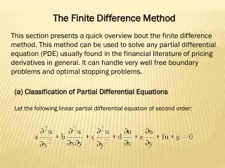
Problem Set Up • Equations used:
Process • Determine (x,y) position of each node • Create finite difference equations for desired set of boundary conditions • Build augmented matrix for solution • Solve matrices for temperatures at each node (matrix inversion) • Build algorithm to automatically generate solution matrix Coefficient Matrix for 1 heat flux
Solution – 1st boundary condition T1 = 35 ℃, T2 = 50 ℃, T3 = 100 ℃, T4 = 50 ℃ 4 divisions 5 divisions 9 divisions
Solution – 2nd boundary condition T1 = 0 ℃, T2 = 50 ℃, T3 = 100 ℃, q”4 = 50 W/m2, k = 15.1 W/m*K 4 divisions 5 divisions 9 divisions
Solution – 3rd boundary condition T1 = 100 ℃, q”2 = 75 W/m2, T3 = 50 ℃, q”4 = -25 W/m2, k = 15.1 W/m*K 4 divisions 5 divisions 9 divisions
Conclusions • Numerical Solution Software is very complex • Setting up equations is the hard part • Matrix increases size on order of divisions squared • Calculations take a long time for large very fine mesh