Download
1 / 24
430 likes | 1.3k Views
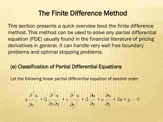
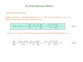
Finite Difference Methods (FDM). FDM. FDM involves three steps: Meshing Approximating PDE & Boundary conditions Computational molecule. Most commonly used grid patterns:. FDM. Forward-difference : Backward-difference: Central-difference: Second derivative:

E N D
FDM • FDM involves three steps: • Meshing • Approximating PDE & Boundary conditions • Computational molecule • Most commonly used grid patterns:
FDM • Forward-difference: • Backward-difference: • Central-difference: • Second derivative: • general approach using Taylor’s series:
FDM • O(x)4is error term. • FDMin x−t: • φ(x,t) at P: • By Central Difference:
FDM ParabolicPDEs • Parabolic PDEs: • Where: • Using: • firsttime row, t=Δt, in terms of boundaryand initialconditions. • secondtime row, t=2Δt, in terms of firsttime row. • Computational Molecule: Circle is unknown Square is known
FDM ParabolicPDEs • Approximations: • Parabolic Implicit formula (Crank-Nicholson1974) • مشتق سمت را با متوسط زمانهای j و j+1 حساب شده است. • Rewritten as: FD = Forward Difference, BD = Backward Difference, CD = Central Difference.
FDM ParabolicPDEs • Example: temperature distribution • Solution: • a rod L=1m, its end ice blocks at 0oC, initially at 100oC, symmetry at x=0.5: • Solution (cont.): • Analytic: • Comparison at x=0.4: • T1: Temperature Distribution Due: 7.16
FDM ParabolicPDEs • Solution by using implicit formula, x=0.2, r=1, Δt =0.04: • Rearrangementφ(i,j +1)fori=1,2,3,4at t=0.04: • for t=0.08: • accuracy can be increased by more points for time step.
Accuracy & Stability • Stability: unincrease magnitude in time. • Accuracy: closeness of approximate to exact. • Errors: Modeling Truncation (Discretization) Round-Off • Modeling: mathematical assumptions (linearity a nonlinear PDE). • Truncation: select a finite terms from infinite series. • such as higher-order terms in Taylor series. • Round off: computations can be done only with a finite precision on a computer. • This error is due to limited size of registers in arithmetic unit of computer. • Round off errors can be minimized by using of double-precision arithmetic. • Minimum Total Error: • To determine stability, error εn , at time step n • amplification factor at time n+1: • For stability: g is amplification factor
Accuracy & Stability • By Von Neumann’s Method for explicit scheme: • or: • Let solution be: • By substituting: • For example: or: or:
FDM HyperbolicPDE • Wave Equation (HyperbolicPDE): • Can be written as: • for stability: r ≤1 • r=1: • Example: • Solution: • Analytical: where: Computational Molecule for arbitrary r≤1 Computational Molecule for r=1
FDM Elliptic PDEs where • Elliptic PDE is Poisson’s equation: • Assuming: • If g(x,y)=0, leads to Laplace’s equation: • Alternative fourth order: = mesh size coefficient computational molecule approximation
FDM Elliptic PDEs • FDM to ellipticPDE leads to a large equations. • Other methods: • Band Matrix Method. • Elimination Methods. • Gauss’s Method. • Cholesky’s Method. • Iterative Methods. • Jacobi’s Method. • Gauss-Seidel Method. • Successive Over-Relaxation (SOR) Method. • Gradient Methods. (the convergence is faster) • Matrix Inversion. • Band Matrix Method: • [A] is a sparse matrix,many zero. • [X] unknown values of φ at free nodes. • [B] known values of at fixed nodes. Appendix D sparse matrix:
FDM Elliptic PDEs • What is drawback of band matrix? • [A] is a sparse (many zero). • For small domains, band matrix is OK. • Size [A] grows with square size x. • 4 x 4= 16 voltage samples: X=[V1, V2, … , V16] • [A]=16x16=256 elements. • For 100x100=10000 voltage samples: [A]=10,000x10,000=100,000,000 V1 V2 V3 V4 V1 V2 V3 V4 • Example: V13 V14 V15 V16
FDM Elliptic PDEs • Iterative Methods: • It is used to solve excessive computational resources • iterative methods are (Appendix D): • Jacobi • Gauss-Seidel • Successive Over Relaxation (SOR) • To apply SOR to equation: • First step is residualR(i,j): • Rk(i, j) at kthiteration is a correction added to φ(i, j). • converging to correct value, Rk(i, j) tends to zero. • ω (relaxation factor) is used to improve rate of convergence: • ωoptmust be found by trial and error: • In order to start: 1<ω<2
FDM Elliptic PDEs • Example: • Solution: • Assuming: • superposition: • V1subject to inhomogeneous conditions. • V2Poisson’s equation homogeneous conditions. • analytical methods: • By SOR, ωopt is smaller root [10]: • T2: Apply SOR, compare with exact Due: 7.23
FDM for Nonrectangular Systems • Cylindrical Coordinates: • Laplace’s equation: • no φdependence: V=V(ρ,z) FDM molecule (1)
FDM for Nonrectangular Systems = • Using: • for Poisson’s case: • interface: D1n=D2n • By apply Taylor series expansion to point 1, 2, 5 in medium 1: other form (1) (2) medium 1
FDM for Nonrectangular Systems • Combining two eq. : • or: • Similarly, Taylor series to 1, 2, and 6 in medium 2: • or: • Using: D1n=D2n • Substituting in two eq: • only for interface points: (2) = (1)if εr1= εr2 (2)
FDM for Nonrectangular Systems • approximations for some boundary points:
FDM for Nonrectangular Systems • Example: (cylindrical case) • an earthed metal cylindrical tank partly filled with a charge liquid (hydrocarbons): • Determine V in entire domain using FDM. • Assume: • Plot V along ρ=0.5, 0<z<2m. • Plot V on surface of liquid. • Exact analytic (section 2.7 Sadiku):
FDM for Nonrectangular Systems • symmetry z-axis: • z-axis is a flux line: ∂V/∂n=∂V/∂ρ=0. • Using FDM: • Δρ=Δz=h=0.05m, 0≤i≤Imax=20, 0≤j≤Jmax=40. • z-axis (i=0) Neumann condition: • Gas= εr1 & liquid=εr2 • Use boundary condition in eq. (2) on liquid-gas interface. along ρ=0.5m,0≤z≤2m eq. 3-120 (Sadiku) along gas-liquid interface • T3: Do and compare results with exact solution. Also p=.9, 0.01 Due: 7.30
FDM for Nonrectangular Systems • Spherical Coordinates: • FDM approximation: computational molecule