Download
1 / 28
280 likes | 526 Views
TSEC-BIOSYS Theme 2 - Topic 2.2 Modelling biomass supply. Contributor: Rothamsted Research 3 rd Annual Meeting Month 40 of 42 November 2008. Modelling bioenergy crops - key objectives. Purpose I is to assess Production potential of bioenergy (BE) at the sub-regional scale,

E N D
TSEC-BIOSYSTheme 2 - Topic 2.2Modelling biomass supply Contributor: Rothamsted Research 3rd Annual Meeting Month 40 of 42 November 2008
Modelling bioenergy crops - key objectives Purpose I is to assess • Production potential of bioenergy (BE) at the sub-regional scale, • Trade-offs of BE vs. Food within land use change (LUC), • Cost-based supply as an option within the UK energy mix, and • Environmental implications, like GHG-balance and hydrology Purpose II is to • Describe, quantify and predict system behaviour • Underpin processes in aide of crop selection/breeding (G x E) • Identify the most important genotypic traits and • Locate crucial control points of yield formation
Task within TSEC-BIOSYS Theme 2: Evolution of UK biomass supply • Topic 2.2: Bioenergy Modelsresources • Biofuel from arable crops – models @ RRES • Winter wheat, sugar beet, • Oilseed rape, maize • Biomass from grasses, mainly Miscanthus • Empirical model for Miscanthus (& switchgrass) • Maps of yield under current climate • Process model for Miscanthus is available; parameterized, calibrated and evaluated; • Ready to be used for predictive purposes
Empirical yield model for MiscanthusRichter, G. M. et al. (2008) Soil Use and Management24 (3), 235
BE Allocation Trade-offs Aide to Producers & LUC planners Economic of BE Supply & Demand Assess environmental impact/benefit Richter et al., Soil Use Manage24, 235 (2008) GHG H20 Application of empirical yield maps
Land use trade-offs - Methods • Incorporated a range of constraints on energy crops • environmental, physical • agricultural, agronomic • socio-economic • Accounted for currently grown food crops • Used Miscanthus yield map for England Lovett, A. A. et al., BioEnergy Research (u. rev.)
Land use trade-offs – Results • Regional contrasts occur in the importance of different constraints • Between 80 and 20% of are below an economic threshold of 9 t/ha • Areas with highest yields co-locate with important food producing areas Lovett, A. A. et al., BioEnergy Research (u.rev.)
Supply & Demand Modelling • Majority of land would yield between 10 - 14 t odm/ha/yr • Cost map gives annual cost of 20 to 60 £/t odm • Switch from yield to cost optimal crop affects only a small fraction of land • Preference map shows 4.4 Mha of Miscanthus and 6 Mha of SRC
Conclusions for integration (Theme 4) - based on working paper between IC, UoSo, RRes, FR • Yield maps are available for Miscanthus, willow and poplar • Overlay of yield maps implied some exclusion criteria (slope > 15%, organic soils) • Yield and cost advantage maps have been created • Potential availability of 10 Mha preferably used for willow and Miscanthus (ratio 6:4) • Suitability and constraint maps reduced area to about 3 Mha (preference of food production given to high grade land) – cooperation with UEA (Lovett) • Simulations of biomass crop allocation based on opportunity costs confirmed expansion of lower grade land being used under higher BE-demand • Paper is based on empirical models describing current (past) yields only – future scenarios (2050) are excluded up to now • Future scenarios must be based on process-based models
Modelling Purpose II • Describe, quantify and predict system behaviour at process-level • Underpin the processes in aide of crop selection and breeding (G x E interaction) • Identify the most important genotypic traits that can be easily quantified and • Locate crucial control points of yield formation
Experimental basis for Process Model • Long-term, highly resolved data at Rothamsted • Light interception (LAI) • Dry matter • Leaf senescence, loss (litter) • Morphological data • Stem number, height & diameter • Leaf length, width • Growth dynamics of belowground biomass (rhizomes) Christian, D. G. et al., Biomass & Bioenergy30, 125 (2006) Christian, D. G., Riche, A. B., Yates, N. E., Industrial Crops and Products28, 109 (2008)
Leaves LAI Stems Density (n), Ht, Wt Rhizomes RGR(T), SRWT, [RhDR(t)] Flowers A sink-source interaction model Physiology Asat, φ rs, ksen,,fW, fT rdr, halflife rad, P, T,.. Photo- synthesis Inter- ception ksen kfrost kext fT(A) Energy Balance Ta PER Phenology Phyllochron, nL Tb, TΣ(e, x, a), cv2g Carbohydrates fw cL/P fsht Tillering Morphology WD(L), SLA, nV, nG MaxHt, SSW(d) Water Balance crf Reserves 10-20% Roots θfc, θpw, depth, ... Source Formation Sink Formation
Parameter sensitivity for Miscanthus • Grouped according to • Initial establishment • Phenology • Physiology • Morphology
500 cL/P 400 kext Asat 300 σ_Change φ fsht cSSW 200 WDL SLAx Tb(A) Tn(A) 100 Tb(sht) physio- pheno- Tx(A) morpho- initial 0 0 500 1000 1500 2000 2500 3000 μ_Change Model evaluation – Sensitivity Analysis Toptv2g DMrhz cv2g TΣ(x)
Model evaluation – shoots • Shoot ≡ Generative Tiller • Initially fixed No. of VegTiller • cv2gis an important factor • Tiller dynamics linked to height • Height dynamics • Increases with GY • PER function of T& CHORes • Partitioning PER using cL/P • Stem weight evaluation • Discrepancy is consequence of height estimate, tiller dynamics • Loss of stem weight at harvest is due to stubble
Conclusions for Process-based Model • A generic grass model was successfully adopted to simulate dry matter production of Miscanthus x giganteus • Identified important morphological traits • Calibrated & evaluated for one site, one variety • Ranked parameter using OAT sensitivity analysis • Exploring sink-source balance, tillering dynamics • Future applications of this model are needed • For different species & varieties to identify optimal grass ideotypes • In different environments (G x E interaction)
T-scale function, photosynthesis Asat, φ = f(Ta) Naidu, S. L. et al., Plant Physiology132 (3), 1688 (2003). Farage, P. K., Blowers, D., Long, S. P., and Baker, N. R., Plant Cell and Environment29 (4), 720 (2006).
Water stress function late response early response Sinclair, T. R., Field Crops Res.15, 125 (1986). Richter, G. M., Jaggard, K. W., Mitchell, R. A. C., Agric For Meteorol109, 13 (2001).
Leaf extension rates (L/PER) A priori parameters from Clifton-Brown & Jones (1997) Simplified either as linear model or Arrhenius function (Q10) Compared to in situ measurements Specific area (SLA) Unchanged principle from LinGra giving a min-max range Range adjusted to observed SLA Dynamic components Number of leaves growing simultaneously (nL 2.7 → > 3) Senescence rates (age, shading, drought) determine tiller density Morphological Parameters – Leaf
Morphological parameters – Shoot/Stem • Stem extension rate • Related to leaf extension rate e.g. le~ 0.83 ±0.07; (Clifton-Brown & Jones 1997) • Shoot density [ m-2 ] • Initially 100 to 140 m-2(Danalatos et al. 2007; Bullard et al. 1995) • 50 to 80 m-2 at equilibrium(Clifton-Brown & Jones 1997; Danalatos et al. 2007) • Specific stem weight • 10 to 11 g m-2 (acc. to Danalatos et al., 2007) • Changes with height and plant age(unpublished)
Sensitivity Analysis • Morris-method varies parameters as one-at-a-time at discrete levels (4 to 8) • Parameters given as mean ± % variation, randomly generated within 5-95% • “change” is defined as Δyield/Δparameter • μ / μ* are means of distribution of the “global” parameter effect • “σ” is an estimate of second- and higher order effects of parameter (interactions with other factors, non-linearity) • Simultaneous display of μ* and σ allows to check for non-monotonic models (negative elements in distribution) References Morris (1991) as described in Saltelli et al. (2004)* Morris M.D. Technometrics 33(2) 161-174; Saltelli A., et al.. Sensitivity analysis in practice. WILEY