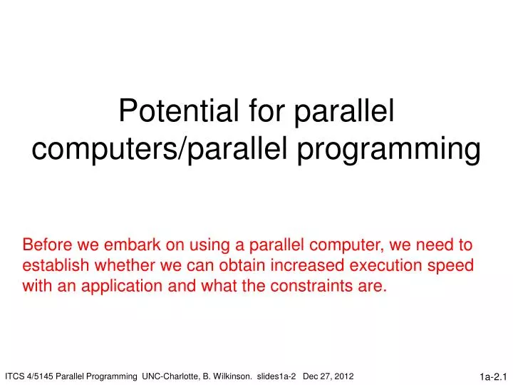
Potential for parallel computers/parallel programming

1. Potential for parallel computers/parallel programming Before we embark on using a parallel computer, we need to establish whether we can obtain increased execution speed with an application and what the constraints are. ITCS 4/5145 Parallel Programming UNC-Charlotte, B. Wilkinson. slides1a-2 Dec 27, 2012

2. Speedup Factor ts Execution time using one processor (best sequential algorithm) S(p) = = tp where ts is execution time on a single processor, and tp is execution time on a multiprocessor. S(p) gives increase in speed by using multiprocessor. Typically use best sequential algorithm for single processor system. Underlying algorithm for parallel implementation might be (and is usually) different. Execution time using a multiprocessor with p processors

3. Parallel time complexity Can extend sequential time complexity notation to parallel computations. Speedup factor can also be cast in terms of computational steps: although several factors may complicate this matter, including: • Individual processors usually do not operate in synchronism and do not perform their steps in unison • Additional message passing overhead Number of computational steps using one processor S(p)= Number of parallel computational steps with p processors

4. Maximum Speedup Maximum speedup usually p with p processors (linear speedup). Possible to get superlinear speedup (greater than p) but usually a specific reason such as: • Extra memory in multiprocessor system • Nondeterministic algorithm

5. Superlinear Speedup example - Searching (a) Searching each sub-space sequentially Start Time t s t /p s Sub-space D t search x t /p s Solution found x indeterminate

6. (b) Searching each sub-space in parallel t s ´ D x + t p S(p) = D t D t • Speed-up: Solution found

7. Worst case for sequential search when solution found in last sub-space search. Greatest benefit for parallel version p – 1 ´ D t + t s p ® ¥ S(p) = D t as Least advantage for parallel version when solution found in first sub-space search of sequential search, i.e. t tends to 0 D Actual speed-up depends upon which subspace holds solution but could be extremely large. D t = 1 S(p) = D t

8. Why superlinear speedup should not be possible in other cases: Without such features as a nondeterministic algorithm or additional memory in parallel computer if we were to get superlinear speed up, then we could argue that the sequential algorithm used is sub-optimal as the parallel parts in parallel algorithm could simply done in sequence on a single computer for a faster sequential solution.

9. Maximum speedup with parts not parallelizable (usual case)Amdahl’s law (circa 1967) t s ft (1 - f ) t s s Serial section Parallelizable sections (a) One processor (b) Multiple processors Note the serial section is bunched at the beginning but in practice may be at the beginning, end, and inbetween p processors (1 - f ) t / p s t p

10. Speedup factor is given by: This equation is known as Amdahl’s law.

11. Speedup against number of processors f = 0% 20 16 12 f = 5% 8 f = 10% f = 20% 4 4 8 12 16 20 Number of processors , p

12. Even with infinite number of processors, maximum speedup limited to 1/f. Example With only 5% of computation being serial, maximum speedup is 20, irrespective of number of processors. This is a very discouraging result. Amdahl used this argument to support the design of ultra-high speed single processor systems in the 1960s.

13. Gustafson’s law Later, Gustafson (1988) described how the conclusion of Amdahl’s law might be overcome by considering the effect of increasing the problem size. He argued that when a problem is ported onto a multiprocessor system, larger problem sizes can be considered, that is, the same problem but with a larger number of data values.

14. Gustafson’s law Starting point for Gustafson’s law is the computation on the multiprocessor rather than on the single computer. In Gustafson’s analysis, parallel execution time kept constant, which we assume to be some acceptable time for waiting for the solution.

15. Gustafson’s law* f ’tp + (1 – f ’)ptp S’(p) = = p - (p – 1)f ’ Using same approach as for Amdahl’s law: Conclusion - almost linear increase in speedup with increasing number of processors, but fractional sequential part f ‘ needs to diminish with increasing problem size. Example: if f ‘ is 5%, scaled speedup is 19.05 with 20 processors whereas with Amdahl’s law and f = 5% speedup is 10.26. Gustafson quotes results obtained in practice of very high speedup close to linear on a 1024-processor hypercube. tp * See Wikipedia http://en.wikipedia.org/wiki/Gustafson%27s_law for original derivation of Gustafson's law.

16. Next question to answer is how does one construct a computer system with multiple processors to achieve the speed-up?