Download
1 / 84
840 likes | 1.14k Views
CS 267: Applications of Parallel Computers Graph Partitioning. James Demmel and Horst Simon www.cs.berkeley.edu/~demmel/cs267_Spr10. Outline of Graph Partitioning Lecture. Review definition of Graph Partitioning problem Overview of heuristics Partitioning with Nodal Coordinates

E N D
CS 267: Applications of Parallel ComputersGraph Partitioning James Demmel and Horst Simon www.cs.berkeley.edu/~demmel/cs267_Spr10 CS267 Lecture 8
Outline of Graph Partitioning Lecture • Review definition of Graph Partitioning problem • Overview of heuristics • Partitioning with Nodal Coordinates • Ex: In finite element models, node at point in (x,y) or (x,y,z) space • Partitioning without Nodal Coordinates • Ex: In model of WWW, nodes are web pages • Multilevel Acceleration • BIG IDEA, appears often in scientific computing • Comparison of Methods and Applications CS267 Lecture 8
Definition of Graph Partitioning • Given a graph G = (N, E, WN, WE) • N = nodes (or vertices), • WN = node weights • E = edges • WE = edge weights • Ex: N = {tasks}, WN = {task costs}, edge (j,k) in E means task j sends WE(j,k) words to task k • Choose a partition N = N1 U N2 U … U NP such that • The sum of the node weights in each Nj is “about the same” • The sum of all edge weights of edges connecting all different pairs Nj and Nk is minimized • Ex: balance the work load, while minimizing communication • Special case of N = N1 U N2: Graph Bisection 2 (2) 1 3 (1) 4 1 (2) 2 4 (3) 3 1 2 2 5 (1) 8 (1) 1 6 5 6 (2) 7 (3) CS267 Lecture 8
Definition of Graph Partitioning • Given a graph G = (N, E, WN, WE) • N = nodes (or vertices), • WN = node weights • E = edges • WE = edge weights • Ex: N = {tasks}, WN = {task costs}, edge (j,k) in E means task j sends WE(j,k) words to task k • Choose a partition N = N1 U N2 U … U NP such that • The sum of the node weights in each Nj is “about the same” • The sum of all edge weights of edges connecting all different pairs Nj and Nk is minimized (shown in black) • Ex: balance the work load, while minimizing communication • Special case of N = N1 U N2: Graph Bisection 2 (2) 1 3 (1) 4 1 (2) 2 4 (3) 3 1 2 2 5 (1) 8 (1) 1 6 5 6 (2) 7 (3) CS267 Lecture 8
Some Applications • Telephone network design • Original application, algorithm due to Kernighan • Load Balancing while Minimizing Communication • Sparse Matrix times Vector Multiplication • Solving PDEs • N = {1,…,n}, (j,k) in E if A(j,k) nonzero, • WN(j) = #nonzeros in row j, WE(j,k) = 1 • VLSI Layout • N = {units on chip}, E = {wires}, WE(j,k) = wire length • Sparse Gaussian Elimination • Used to reorder rows and columns to increase parallelism, and to decrease “fill-in” • Data mining and clustering • Physical Mapping of DNA • Image Segmentation CS267 Lecture 8
Sparse Matrix Vector Multiplication y = y +A*x … declare A_local, A_remote(1:num_procs), x_local, x_remote, y_local y_local = y_local + A_local * x_local for all procs P that need part of x_local send(needed part of x_local, P) for all procs P owning needed part of x_remote receive(x_remote, P) y_local = y_local + A_remote(P)*x_remote CS267 Lecture 8
Cost of Graph Partitioning • Many possible partitionings to search • Just to divide in 2 parts there are: n choose n/2 = n!/((n/2)!)2 ~ sqrt(2/(np))*2npossibilities • Choosing optimal partitioning is NP-complete • (NP-complete = we can prove it is a hard as other well-known hard problems in a class Nondeterministic Polynomial time) • Only known exact algorithms have cost = exponential(n) • We need good heuristics CS267 Lecture 8
Outline of Graph Partitioning Lectures • Review definition of Graph Partitioning problem • Overview of heuristics • Partitioning with Nodal Coordinates • Ex: In finite element models, node at point in (x,y) or (x,y,z) space • Partitioning without Nodal Coordinates • Ex: In model of WWW, nodes are web pages • Multilevel Acceleration • BIG IDEA, appears often in scientific computing • Comparison of Methods and Applications CS267 Lecture 8
First Heuristic: Repeated Graph Bisection • To partition N into 2k parts • bisect graph recursively k times • Henceforth discuss mostly graph bisection CS267 Lecture 8
Edge Separators vs. Vertex Separators • Edge Separator: Es (subset of E) separates G if removing Es from E leaves two ~equal-sized, disconnected components of N: N1 and N2 • Vertex Separator: Ns (subset of N) separates G if removing Ns and all incident edges leaves two ~equal-sized, disconnected components of N: N1 and N2 • Making an Ns from an Es: pick one endpoint of each edge in Es • |Ns| |Es| • Making an Es from an Ns: pick all edges incident on Ns • |Es| d * |Ns| where d is the maximum degree of the graph • We will find Edge or Vertex Separators, as convenient G = (N, E), Nodes N and Edges E Es = green edges or blue edges Ns = red vertices CS267 Lecture 8
Overview of Bisection Heuristics • Partitioning with Nodal Coordinates • Each node has x,y,z coordinates partition space • Partitioning without Nodal Coordinates • E.g., Sparse matrix of Web documents • A(j,k) = # times keyword j appears in URL k • Multilevel acceleration (BIG IDEA) • Approximate problem by “coarse graph,” do so recursively CS267 Lecture 8
Outline of Graph Partitioning Lectures • Review definition of Graph Partitioning problem • Overview of heuristics • Partitioning with Nodal Coordinates • Ex: In finite element models, node at point in (x,y) or (x,y,z) space • Partitioning without Nodal Coordinates • Ex: In model of WWW, nodes are web pages • Multilevel Acceleration • BIG IDEA, appears often in scientific computing • Comparison of Methods and Applications CS267 Lecture 8
Nodal Coordinates: How Well Can We Do? • A planar graph can be drawn in plane without edge crossings • Ex: m x m grid of m2 nodes: $ vertex separatorNs with |Ns| = m = sqrt(|N|) (see earlier slide for m=5 ) • Theorem (Tarjan, Lipton, 1979): If G is planar, $ Ns such that • N = N1 U Ns U N2 is a partition, • |N1| <= 2/3 |N| and |N2| <= 2/3 |N| • |Ns| <= sqrt(8 * |N|) • Theorem motivates intuition of following algorithms CS267 Lecture 8
Choose a line L through the points • L given by a*(x-xbar)+b*(y-ybar)=0, • with a2+b2=1; (a,b) is unit vector ^ to L L • Project each point to the line • For each nj = (xj,yj), compute coordinate • Sj = -b*(xj-xbar) + a*(yj-ybar) along L • Compute the median • Let Sbar = median(S1,…,Sn) (xbar,ybar) (a,b) • Use median to partition the nodes • Let nodes with Sj < Sbar be in N1, rest in N2 Nodal Coordinates: Inertial Partitioning • For a graph in 2D, choose line with half the nodes on one side and half on the other • In 3D, choose a plane, but consider 2D for simplicity • Choose a line L, and then choose a line L^ perpendicular to it, with half the nodes on either side L^ CS267 Lecture 8
Inertial Partitioning: Choosing L • Clearly prefer L, L^ on left below • Mathematically, choose L to be a total least squares fit of the nodes • Minimize sum of squares of distances to L (green lines on last slide) • Equivalent to choosing L as axis of rotation that minimizes the moment of inertia of nodes (unit weights) - source of name L N1 N1 N2 L L^ N2 L^ CS267 Lecture 8
L (xbar,ybar) (a,b) Inertial Partitioning: choosing L (continued) (xj , yj ) (a,b) is unit vector perpendicular to L Sj (length of j-th green line)2 = Sj [ (xj - xbar)2 + (yj - ybar)2 - (-b*(xj - xbar) + a*(yj - ybar))2 ] … Pythagorean Theorem = a2 * Sj (xj - xbar)2 + 2*a*b* Sj (xj - xbar)*(xj - ybar) + b2Sj (yj - ybar)2 = a2 * X1 + 2*a*b* X2 + b2 * X3 = [a b] * X1 X2 * a X2 X3 b Minimized by choosing (xbar , ybar) = (Sj xj , Sj yj) / n = center of mass (a,b) = eigenvector of smallest eigenvalue of X1 X2 X2 X3 CS267 Lecture 8
Nodal Coordinates: Random Spheres • Generalize nearest neighbor idea of a planar graph to higher dimensions • Any graph can fit in 3D without edge crossings • Capture intuition of planar graphs of being connected to “nearest neighbors” but in higher than 2 dimensions • For intuition, consider graph defined by a regular 3D mesh • An n by n by n mesh of |N| = n3 nodes • Edges to 6 nearest neighbors • Partition by taking plane parallel to 2 axes • Cuts n2 =|N|2/3 = O(|E|2/3) edges • For the general graphs • Need a notion of “well-shaped” like mesh CS267 Lecture 8
Random Spheres: Well Shaped Graphs • Approach due to Miller, Teng, Thurston, Vavasis • Def: A k-ply neighborhood system in d dimensions is a set {D1,…,Dn} of closed disks in Rd such that no point in Rd is strictly interior to more than k disks • Def: An (a,k) overlap graph is a graph defined in terms of a 1 and a k-ply neighborhood system {D1,…,Dn}: There is a node for each Dj, and an edge from j to i if expanding the radius of the smaller of Dj and Di by >a causes the two disks to overlap Ex: n-by-n mesh is a (1,1) overlap graph Ex: Any planar graph is (a,k) overlap for some a,k 2D Mesh is (1,1) overlap graph CS267 Lecture 8
Generalizing Lipton/Tarjan to Higher Dimensions • Theorem (Miller, Teng, Thurston, Vavasis, 1993): Let G=(N,E) be an (a,k) overlap graph in d dimensions with n=|N|. Then there is a vertex separator Ns such that • N = N1 U Ns U N2 and • N1 and N2 each has at most n*(d+1)/(d+2) nodes • Ns has at most O(a * k1/d * n(d-1)/d ) nodes • When d=2, same as Lipton/Tarjan • Algorithm: • Choose a sphere S in Rd • Edges that S “cuts” form edge separator Es • Build Ns from Es • Choose S “randomly”, so that it satisfies Theorem with high probability CS267 Lecture 8
Stereographic Projection • Stereographic projection from plane to sphere • In d=2, draw line from p to North Pole, projection p’ of p is where the line and sphere intersect • Similar in higher dimensions p’ p p = (x,y) p’ = (2x,2y,x2 + y2 –1) / (x2 + y2 + 1) CS267 Lecture 8
Choosing a Random Sphere • Do stereographic projection from Rd to sphere S in Rd+1 • Find centerpoint of projected points • Any plane through centerpoint divides points ~evenly • There is a linear programming algorithm, cheaper heuristics • Conformally map points on sphere • Rotate points around origin so centerpoint at (0,…0,r) for some r • Dilate points (unproject, multiply by sqrt((1-r)/(1+r)), project) • this maps centerpoint to origin (0,…,0), spreads points around S • Pick a random plane through origin • Intersection of plane and sphere S is “circle” • Unproject circle • yields desired circle C in Rd • Create Ns: j belongs to Ns if a*Dj intersects C CS267 Lecture 8
Random Sphere Algorithm (Gilbert) CS267 Lecture 23
Random Sphere Algorithm (Gilbert) CS267 Lecture 23
Random Sphere Algorithm (Gilbert) CS267 Lecture 23
Random Sphere Algorithm (Gilbert) CS267 Lecture 8
Random Sphere Algorithm (Gilbert) CS267 Lecture 23
Random Sphere Algorithm (Gilbert) CS267 Lecture 23
Nodal Coordinates: Summary • Other variations on these algorithms • Algorithms are efficient • Rely on graphs having nodes connected (mostly) to “nearest neighbors” in space • algorithm does not depend on where actual edges are! • Common when graph arises from physical model • Ignores edges, but can be used as good starting guess for subsequent partitioners that do examine edges • Can do poorly if graph connection is not spatial: • Details at • www.cs.berkeley.edu/~demmel/cs267/lecture18/lecture18.html • www.cs.ucsb.edu/~gilbert • www.cs.bu.edu/~steng CS267 Lecture 8
Outline of Graph Partitioning Lectures • Review definition of Graph Partitioning problem • Overview of heuristics • Partitioning with Nodal Coordinates • Ex: In finite element models, node at point in (x,y) or (x,y,z) space • Partitioning without Nodal Coordinates • Ex: In model of WWW, nodes are web pages • Multilevel Acceleration • BIG IDEA, appears often in scientific computing • Comparison of Methods and Applications CS267 Lecture 8
Coordinate-Free: Breadth First Search (BFS) • Given G(N,E) and a root node r in N, BFS produces • A subgraph T of G (same nodes, subset of edges) • T is a tree rooted at r • Each node assigned a level = distance from r root Level 0 Level 1 Level 2 Level 3 Level 4 N1 N2 Tree edges Horizontal edges Inter-level edges CS267 Lecture 8
root Breadth First Search • Queue (First In First Out, or FIFO) • Enqueue(x,Q) adds x to back of Q • x = Dequeue(Q) removes x from front of Q • Compute Tree T(NT,ET) NT = {(r,0)}, ET = empty set … Initially T = root r, which is at level 0 Enqueue((r,0),Q) … Put root on initially empty Queue Q Mark r … Mark root as having been processed While Q not empty … While nodes remain to be processed (n,level) = Dequeue(Q) … Get a node to process For all unmarked children c of n NT = NT U (c,level+1) … Add child c to NT ET = ET U (n,c) … Add edge (n,c) to ET Enqueue((c,level+1),Q)) … Add child c to Q for processing Mark c … Mark c as processed Endfor Endwhile CS267 Lecture 8
root Partitioning via Breadth First Search • BFS identifies 3 kinds of edges • Tree Edges - part of T • Horizontal Edges - connect nodes at same level • Interlevel Edges - connect nodes at adjacent levels • No edges connect nodes in levels differing by more than 1 (why?) • BFS partioning heuristic • N = N1 U N2, where • N1 = {nodes at level <= L}, • N2 = {nodes at level > L} • Choose L so |N1| close to |N2| BFS partition of a 2D Mesh using center as root: N1 = levels 0, 1, 2, 3 N2 = levels 4, 5, 6 CS267 Lecture 8
Coordinate-Free: Kernighan/Lin • Take a initial partition and iteratively improve it • Kernighan/Lin (1970), cost = O(|N|3) but easy to understand • Fiduccia/Mattheyses (1982), cost = O(|E|), much better, but more complicated • Given G = (N,E,WE) and a partitioning N = A U B, where |A| = |B| • T = cost(A,B) = S {W(e) where e connects nodes in A and B} • Find subsets X of A and Y of B with |X| = |Y| • Consider swapping X and Y if it decreases cost: • newA = (A – X) U Y and newB = (B – Y) U X • newT = cost(newA , newB) < T = cost(A,B) • Need to compute newT efficiently for many possible X and Y, choose smallest (best) CS267 Lecture 8
Kernighan/Lin: Preliminary Definitions • T = cost(A, B), newT = cost(newA, newB) • Need an efficient formula for newT; will use • E(a) = external cost of a in A = S {W(a,b) for b in B} • I(a) = internal cost of a in A = S {W(a,a’) for other a’ in A} • D(a) = cost of a in A = E(a) - I(a) • E(b), I(b) and D(b) defined analogously for b in B • Consider swapping X = {a} and Y = {b} • newA = (A - {a}) U {b}, newB = (B - {b}) U {a} • newT = T - ( D(a) + D(b) - 2*w(a,b) ) ≡ T - gain(a,b) • gain(a,b) measures improvement gotten by swapping a and b • Update formulas • newD(a’) = D(a’) + 2*w(a’,a) - 2*w(a’,b) for a’ in A, a’ ≠ a • newD(b’) = D(b’) + 2*w(b’,b) - 2*w(b’,a) for b’ in B, b’ ≠ b CS267 Lecture 8
Kernighan/Lin Algorithm Compute T = cost(A,B) for initial A, B … cost = O(|N|2) Repeat … One pass greedily computes |N|/2 possible X,Y to swap, picks best Compute costs D(n) for all n in N … cost = O(|N|2) Unmark all nodes in N … cost = O(|N|) While there are unmarked nodes … |N|/2 iterations Find an unmarked pair (a,b) maximizing gain(a,b) … cost = O(|N|2) Mark a and b (but do not swap them) … cost = O(1) Update D(n) for all unmarked n, as though a and b had been swapped … cost = O(|N|) Endwhile … At this point we have computed a sequence of pairs … (a1,b1), … , (ak,bk) and gains gain(1),…., gain(k) … where k = |N|/2, numbered in the order in which we marked them Pick m maximizing Gain = Sk=1 to m gain(k) … cost = O(|N|) … Gain is reduction in cost from swapping (a1,b1) through (am,bm) If Gain > 0 then … it is worth swapping Update newA = A - { a1,…,am } U { b1,…,bm } … cost = O(|N|) Update newB = B - { b1,…,bm } U { a1,…,am } … cost = O(|N|) Update T = T - Gain … cost = O(1) endif Until Gain <= 0 CS267 Lecture 8
Comments on Kernighan/Lin Algorithm • Most expensive line shown in red, O(n3) • Some gain(k) may be negative, but if later gains are large, then final Gain may be positive • can escape “local minima” where switching no pair helps • How many times do we Repeat? • K/L tested on very small graphs (|N|<=360) and got convergence after 2-4 sweeps • For random graphs (of theoretical interest) the probability of convergence in one step appears to drop like 2-|N|/30 CS267 Lecture 8
Coordinate-Free: Spectral Bisection • Based on theory of Fiedler (1970s), popularized by Pothen, Simon, Liou (1990) • Motivation, by analogy to a vibrating string • Basic definitions • Vibrating string, revisited • Implementation via the Lanczos Algorithm • To optimize sparse-matrix-vector multiply, we graph partition • To graph partition, we find an eigenvector of a matrix associated with the graph • To find an eigenvector, we do sparse-matrix vector multiply • No free lunch ... CS267 Lecture 8
Motivation for Spectral Bisection • Vibrating string • Think of G = 1D mesh as masses (nodes) connected by springs (edges), i.e. a string that can vibrate • Vibrating string has modes of vibration, or harmonics • Label nodes by whether mode - or + to partition into N- and N+ • Same idea for other graphs (eg planar graph ~ trampoline) CS267 Lecture 8
Basic Definitions • Definition: The incidence matrix In(G) of a graph G(N,E) is an |N| by |E| matrix, with one row for each node and one column for each edge. If edge e=(i,j) then column e of In(G) is zero except for the i-th and j-th entries, which are +1 and -1, respectively. • Slightly ambiguous definition because multiplying column e of In(G) by -1 still satisfies the definition, but this won’t matter... • Definition: The Laplacian matrix L(G) of a graph G(N,E) is an |N| by |N| symmetric matrix, with one row and column for each node. It is defined by • L(G) (i,i) = degree of node i (number of incident edges) • L(G) (i,j) = -1 if i ≠ j and there is an edge (i,j) • L(G) (i,j) = 0 otherwise CS267 Lecture 8
Example of In(G) and L(G) for Simple Meshes CS267 Lecture 8
Properties of Laplacian Matrix • Theorem 1: Given G, L(G) has the following properties (proof on 1996 CS267 web page) • L(G) is symmetric. • This means the eigenvalues of L(G) are real and its eigenvectors are real and orthogonal. • In(G) * (In(G))T = L(G) • The eigenvalues of L(G) are nonnegative: • 0 = l1l2 … ln • The number of connected components of G is equal to the number of li equal to 0. • Definition: l2(L(G)) is the algebraic connectivity of G • The magnitude of l2 measures connectivity • In particular, l2≠ 0 if and only if G is connected. CS267 Lecture 8
Spectral Bisection Algorithm • Spectral Bisection Algorithm: • Compute eigenvector v2 corresponding to l2(L(G)) • For each node n of G • if v2(n) < 0 put node n in partition N- • else put node n in partition N+ • Why does this make sense? First reasons... • Theorem 2 (Fiedler, 1975): Let G be connected, and N- and N+ defined as above. Then N- is connected. If no v2(n) = 0, then N+ is also connected. (proof on 1996 CS267 web page) • Recall l2(L(G)) is the algebraic connectivity of G • Theorem 3 (Fiedler): Let G1(N,E1) be a subgraph of G(N,E), so that G1 is “less connected” than G. Then l2(L(G1)) l2(L(G)) , i.e. the algebraic connectivity of G1 is less than or equal to the algebraic connectivity of G. (proof on 1996 CS267 web page) CS267 Lecture 8
Spectral Bisection Algorithm • Spectral Bisection Algorithm: • Compute eigenvector v2 corresponding to l2(L(G)) • For each node n of G • if v2(n) < 0 put node n in partition N- • else put node n in partition N+ • Why does this make sense? More reasons... • Theorem 4 (Fiedler, 1975): Let G be connected, and N1 and N2 be any partition into part of equal size |N|/2. Then the number of edges connecting N1 and N2 is at least .25 * |N| * l2(L(G)). (proof on 1996 CS267 web page) CS267 Lecture 8
Motivation for Spectral Bisection (recap) • Vibrating string has modes of vibration, or harmonics • Modes computable as follows • Model string as masses connected by springs (a 1D mesh) • Write down F=ma for coupled system, get matrix A • Eigenvalues and eigenvectors of A are frequencies and shapes of modes • Label nodes by whether mode - or + to get N- and N+ • Same idea for other graphs (eg planar graph ~ trampoline) CS267 Lecture 23
Details for Vibrating String Analogy • Force on mass j = k*[x(j-1) - x(j)] + k*[x(j+1) - x(j)] = -k*[-x(j-1) + 2*x(j) - x(j+1)] • F=ma yields m*x’’(j) = -k*[-x(j-1) + 2*x(j) - x(j+1)] (*) • Writing (*) for j=1,2,…,n yields x(1) 2*x(1) - x(2) 2 -1 x(1) x(1) x(2) -x(1) + 2*x(2) - x(3) -1 2 -1 x(2) x(2) m * d2 … =-k* … =-k* … * … =-k*L* … dx2 x(j) -x(j-1) + 2*x(j) - x(j+1) -1 2 -1 x(j) x(j) … … … … … x(n) 2*x(n-1) - x(n) -1 2 x(n) x(n) (-m/k) x’’ = L*x CS267 Lecture 23
Details for Vibrating String (continued) • -(m/k) x’’ = L*x, where x = [x1,x2,…,xn ]T • Seek solution of form x(t) = sin(a*t) * x0 • L*x0 = (m/k)*a2 * x0 = l * x0 • For each integer i, get l = 2*(1-cos(i*p/(n+1)), x0 = sin(1*i*p/(n+1)) sin(2*i*p/(n+1)) … sin(n*i*p/(n+1)) • Thus x0 is a sine curve with frequency proportional to i • Thus a2 = 2*k/m *(1-cos(i*p/(n+1)) or a ~ sqrt(k/m)*p*i/(n+1) • L = 2 -1 not quite Laplacian of 1D mesh, -1 2 -1 but we can fix that ... …. -1 2 CS267 Lecture 8
Motivation for Spectral Bisection • Vibrating string has modes of vibration, or harmonics • Modes computable as follows • Model string as masses connected by springs (a 1D mesh) • Write down F=ma for coupled system, get matrix A • Eigenvalues and eigenvectors of A are frequencies and shapes of modes • Label nodes by whether mode - or + to get N- and N+ • Same idea for other graphs (eg planar graph ~ trampoline) CS267 Lecture 8
Eigenvectors of L(1D mesh) Eigenvector 1 (all ones) Eigenvector 2 Eigenvector 3 CS267 Lecture 8
2nd eigenvector of L(planar mesh) CS267 Lecture 8
4th eigenvector of L(planar mesh) CS267 Lecture 8