Download
1 / 99
1k likes | 1.16k Views
Optimizing Parallel Embedded Systems Dr. Edwin Sha Professor Computer Science University of Texas at Dallas http://www.utdallas.edu/~edsha edsha@utdallas.edu. Parallel Architecture is Ubiquitous. Parallel Architecture is everywhere As small as cellular phone

E N D
Optimizing Parallel Embedded SystemsDr. Edwin ShaProfessorComputer ScienceUniversity of Texas at Dallashttp://www.utdallas.edu/~edshaedsha@utdallas.edu
Parallel Architecture is Ubiquitous • Parallel Architecture is everywhere • As small as cellular phone • Modern DSP processor (VLIW), network processors • Modern CPU (instruction-level parallelism) • Your home PC (small number of processors) • Application-specific systems (image processing, speech processing, network routers, look-up table, etc.) • File server • Database server or web server • Supercomputers Interested in domain-specific HW/SW parallel systems
Organization of the Presentation • Introduction to parallel architectures • Using sorting as an example to show various implementations on parallel architectures. • Introduction to embedded systems: strict constraints • Timing optimization: parallelize loops and nested loops. • Retiming, Multi-dimensional Retiming • Full Parallelism: all the nodes can be executed in parallel • Design space exploration and optimizations for code size, data memory, low-power, etc. • Intelligent prefetching and partitioning to hide memory latency • Conclusions
Technology Trend • Microprocessor performance increases 50% - 100% per year • Where does the performance gain from? Clock Rate and Capacity. • Clock Rate increases only 30% per year
Technology Trend • Transistor count grows much faster than clock rate. • Increase 40% per year, • Order of magnitude more contribution in 2 decades
Exploit Parallelism at Every Level • Algorithms Level • Thread level • Eg. Each request of service is created as a thread • Iteration level (loop level) • Eg. For_all i= 1 to n do {loop body}. • All n iterations can be parallelized. • Loop body level (instruction-level) • Parallelize instructions inside a loop body as mush as possible • Hardware level: parallelize and pipeline the execution of an instruction such as multiplication, etc.
Sorting on Linear Array of Processors • Input: x1, x2, .. xn. Output: A sorted sequence (Ascending order) • Architecture: a linear array of k processors. Assume k=n at first. • What is the optimal time for sorting. Obviously it takes O(n) time to reach the rightmost. • Lets consider the different sequential algorithms and then think how to use them on a linear array of processors. This is a good example. • Selection Sort • Insertion Sort • Bubble Sort • Bucket Sort • Sample Sort
n(n-1) Timing: (n-1) + … + 2 + 1 = 2 3 + 2 + 1 = 6 5 Selection Sort • Algorithm:for i = 1 to n • pick the ith smallest one 5,1,2,4 Is it good? Keep 1 5,2,4 Keep 2 5,4 Keep 4
Insertion Sort 5,1,2,4 1 2 3 4 Timing:nonly ! 5 1 1 1 4 clock cycles in this example 5 2 2 Problem: Need global bus 5 4 5 time
Systolic array x y Initially, y = If x > y z x else z y y x z Pipeline Sorting without Global Wire Organization
1 1 1 5 4 1 2 1 2 5 1 2 5 5 2 5 5 4 4 2 4 5 Bubble Sorting The worst algorithm in sequential model ! But a good one in this case. 7 clock cycles In this example How about n ? Timing: 2n-1 for n procs. O(n) time O(n n / k) for k procs. Can we get O(n/k log n/k) time
But it assumes n elements are uniformly distributed over an interval [a, b]. • The interval [a, b] is divided into k equal-sized subintervals called buckets. • Scan through each element and put it to the corresponding bucket. The number of elements in each bucket is about n/k. 125 167 102 … 201 257 207 … 399 336 318 … 19 5 98 … 1 400 100 300 -- splitters 200 Bucket Sort • can be lower than the lower bound (n log n) to be O(n)?
Bucket Sort • Then sort each bucket locally. • The sequential running time is O(n + k(n/k) log (n/k)) = O(n log (n/k)). • If k = n/128, then we get O(n) algorithm. • Parallelization is straightforward. • It is pretty good. Very little communication required between processors. • But what happens when the input data are not uniformly distributed. One bucket may have almost all the elements. • How to smartly pick appropriate splitters so each bucket will have at most 2 n/k elements. (Sample sort)
Sample Sort • First Step:Splitter selection(An important step) • Smartly select k-1 splitters from some samples. • Second Step: Bucket sort using these splitters on k buckets. • Guarantee: Each bucket has at most 2n/k elements. • Directly divide n input elements into k blocks of size n/k each and sort each block. • From each sorted block it chooses k-1 evenly spaced elements. Then sort these k(k-1) elements. • Select the k-1 evenly spaced elements from these k(k-1) elements. • Scan through the n input elements and use these k-1 splitters to put each element to the corresponding bucket.
Sample Sort • Sequential: O(n log n/k) + O(k k log k) + O(n log n/k). • Not an O(n) alg. But it is very efficient for parallel implementation Sort Sort Step 1 Sort Sort Sort Step 2 Final splitters Step 3 Bucket sort using these splitters
Randomized Sample Sort • Processor 0 randomly pick d´ k samples. d : over-sampling ratio such as 64 or 128. • Sort these samples and select k-1 evenly spaced numbers as splitters. • With high probability, the splitters are picked well. I.e. with low probability, there is a big bucket. • But cannot be used for hard real-time systems. • To sort 5 million numbers in a SUN cluster with 4 machines using MPI in our tests: • Randomized sample sort takes 5 seconds • Deterministic sample sort takes 10 seconds • Radix sort takes > 500 seconds (too many communications).
Embedded Systems Overview • Embedded computing systems • Computing systems embedded within electronic devices • Repeatedly carry out a particular function or a set of functions. • Nearly any computing system other than a desktop computer are embedded systems • Billions of units produced yearly, versus millions of desktop units • About 50 per household, 50 - 100 per automobile
Some common characteristics of embedded systems • Application Specific • Executes a single program, repeatedly • New ones might be adaptive, and/or multiple mode • Tightly-constrained • Low cost, low power, small, fast, etc. • Reactive and real-time • Continually reacts to changes in the system’s environment • Must compute certain results in real-time without delay
Anti-lock brakes Auto-focus cameras Automatic teller machines Automatic toll systems Automatic transmission Avionic systems Battery chargers Camcorders Cell phones Cell-phone base stations Cordless phones Cruise control Curbside check-in systems Digital cameras Disk drives Electronic card readers Electronic instruments Electronic toys/games Factory control Fax machines Fingerprint identifiers Home security systems Life-support systems Medical testing systems Modems MPEG decoders Network cards Network switches/routers On-board navigation Pagers Photocopiers Point-of-sale systems Portable video games Printers Satellite phones Scanners Smart ovens/dishwashers Speech recognizers Stereo systems Teleconferencing systems Televisions Temperature controllers Theft tracking systems TV set-top boxes VCR’s, DVD players Video game consoles Video phones Washers and dryers A “short list” of embedded systems • And the list grows longer each year.
Digital camera chip CCD CCD preprocessor Pixel coprocessor D2A A2D lens JPEG codec Microcontroller Multiplier/Accum DMA controller Display ctrl Memory controller ISA bus interface UART LCD ctrl An embedded system example -- a digital camera • Single-functioned -- always a digital camera • Tightly-constrained -- Low cost, low power, small, fast
Expertise with both software and hardware is needed to optimize design metrics Not just a hardware or software expert, as is common A designer must be comfortable with various technologies in order to choose the best for a given application and constraints Need serious Design Space Explorations Power Performance Size NRE cost Design metric competition -- improving one may worsen others
Processor technology • Processors vary in their customization for the problem at hand total = 0 for i = 1 to N loop total += M[i] end loop Desired functionality General-purpose processor (software) Application-specific processor Single-purpose processor (hardware)
10,000 100,000 1,000 10,000 100 1000 Logic transistors per chip (in millions) Gap Productivity (K) Trans./Staff-Mo. 10 100 IC capacity 1 10 0.1 1 productivity 0.01 0.1 0.001 0.01 1981 1983 1985 1987 1989 1991 1993 1995 1997 1999 2001 2003 2005 2007 2009 Design Productivity Gap • 1981 leading edge chip required 100 designer months • 10,000 transistors / 100 transistors/month • 2002 leading edge chip requires 30,000 designer months • 150,000,000 / 5000 transistors/month • Designer cost increase from $1M to $300M
More challenges coming • Parallel • Consist of multiple processors with hardware. • Heterogeneous, Networked • Each processor has its own speed, memory, power, reliability, etc. • Fault-Tolerance, Reliability & Security • A major issue for critical applications • Design Space Explorations: timing, code-size, data memory, power consumption, cost, etc. • System-Level Design, Analysis, and Optimization are important. • Compiler is playing an important role. We need more research. • Lets start with Timing optimizations, then other optimizations, and design space issues.
Timing Optimization • Parallelization for Nested Loops • Focus on computation or data intensive applications. • Loops are the most critical parts. • Multi-dimensional systems (MD) Uniform nested loops. • Develop efficient algorithms to obtain the schedule with the minimum execution time while hiding memory latencies. • ALU part: MD Retiming to fully parallelize computations. • Memory part: prefetching and partitioning to hide memory latencies. • Developed by Edwin Sha’s group. The results are exciting.
Graph Representation for Loops • A[0] = A[1] = 0; • For (i=2; i<n; i++) • { • A[i] = D[i-2] / 3; • B[i] = A[i] * 5; • C[i] = A[i] + 7; • D[i] = B[i] + C[i]; • } B A D C Delays
A B C D B A D A B C D C A B C D A B C D … … Schedule looped DFG • DFG: Static Schedule: Schedule Length = 3
A B C D A A B C D A B C D B C D A A B C D A B C D B C D A A B C D A B C D B C D A A B C D A B C D … … B C D … … … … Rotation: Loop pipelining • Original Schedule: Regrouped Schedule: Rotated Schedule: prologue epilogue
B A D C Graph Representation Using Retiming DAG Longest path = 3 B Longest path = 2 A D C
Multi-dimensional Problems: Multi-dimensional problems DO 10 J = 0, N DO 1 I = 0, M d(i,j) = b(i,j-1) * c(i-1,j) D a(i,j) = d(i,j) * .5 A b(i,j) = a(i,j) + 1. B c(i,j) = a(i,j) + 2. C 1 Continue 10 Continue Circuit optimization z2-1 (0,1) B A D z1-1 C (1,0)
An Example of DSP Processor: TI TMS320C64X • Clocking speed: 1.1 GHz, Up to 8800 MIPS.
For I = 1, ….. × 1.3 One-Dimensional Retiming (Leiserson-Saxe, ’91) For I = 1, ….. × 1.3
A(1) = B(-1) + 1 For I = 1, …… B(I) = A(I) × 1.3 A(I+1) = B(I-1) + 1 Another Example For I = 1, ……. × 1.3
Retiming • An integer-value transformation on nodes • Registers are re-distributed • G = < V, E, d > Gr = < V, E, dr > • dr(e) = d(e) + r(u) – r(u)>= 0 Legal retiming # delays of a cycle remains constant
Multi-Dimensional Retiming • A nested loop • Illegal cases • Retiming nested loops • New problems …
Multi-Dimensional Retiming Iteration Space
Iteration Space for Retimed Graph Legal schedule with row-wise executions. S=(0,1)
Required Solution Needs: • To avoid illegal retiming • To be general • To obtain full parallelism • To be a fast Algorithm
Schedule Vector(wavefront processing) Legal schedule: s·d 0
Schedule-Based MD Retiming Legal Feasible
Chained MD Retiming Schedule plane S+ y s • (1,1) > 0 s • (-1,1) > 0 Pick s = (0,1), r s => r = (1,0) s (-1,1) (1,1) x r