Download
1 / 39
400 likes | 498 Views
Correlation and Covariance. Overview. Outcome, Dependent Variable (Y-Axis). Height. Continuous. Histogram. Predictor Variable (X-Axis). Scatter. Continuous. Boxplot. Categorical. Variables. Dependent Variables. Y. Y. Height. X4. X3. X1. X2. Independent Variables. X’s.

E N D
Overview Outcome, Dependent Variable (Y-Axis) Height Continuous Histogram Predictor Variable (X-Axis) Scatter Continuous Boxplot Categorical
Variables Dependent Variables Y Y Height X4 X3 X1 X2 Independent Variables X’s
Correlation Matrix for Continuous Variables PerformanceAnalytics package chart.Correlation(num2)
Calculating ‘Error’ • A deviation is the difference between the mean and an actual data point. • Deviations can be calculated by taking each score and subtracting the mean from it:
Use the Total Error? Deviation • Take the error between the mean and the data and add them????
Deviation Sum of Squared Errors • We could add the deviations to find out the total error. • Deviations cancel out because some are positive and others negative. • Therefore, we square each deviation. • If we add these squared deviations we get the sum of squared errors (SS).
Standard Deviation • The variance is measured in units squared. • This isn’t a very meaningful metric so we take the square root value. • This is the standard deviation(s).
Variance • The sum of squares is a good measure of overall variability, but is dependent on the number of scores. • We calculate the average variability by dividing by the number of scores (n). • This value is called the variance(s2).
Temperature Variation Across Cities Austin Las Vegas San Diego San Francisco Tampa Bay Count of Hours
Covariance Y X Persons 2,3, and 5 look to have similar magnitudes from their means
Covariance • Calculate the error [deviation] between the mean and each subject’s score for the first variable (x). • Calculate the error [deviation] between the mean and their score for the second variable (y). • Multiply these error values. • Add these values and you get the cross product deviations. • The covariance is the average cross-product deviations:
Covariance Do they VARY the same way relative to their own means? 2.47
Limitations of Covariance • It depends upon the units of measurement. • E.g. the covariance of two variables measured in miles might be 4.25, but if the same scores are converted to kilometres, the covariance is 11. • One solution: standardize it! normalize the data • Divide by the standard deviations of both variables. • The standardized version of covariance is known as the correlation coefficient. • It is relatively unaffected by units of measurement.
Things to Know about the Correlation • It varies between -1 and +1 • 0 = no relationship • It is an effect size • ±.1 = small effect • ±.3 = medium effect • ±.5 = large effect • Coefficient of determination, r2 • By squaring the value of r you get the proportion of variance in one variable shared by the other.
Correlation Covariance is High: r ~1 Covariance is Low: r ~0
Correlation Need inter-item/variable correlations > .30
Data Structures character vector numeric vector Dataframe: d <- c(1,2,3,4)e <- c("red", "white", "red", NA)f <- c(TRUE,TRUE,TRUE,FALSE)mydata <- data.frame(d,e,f)names(mydata) <- c("ID","Color","Passed") List: w <- list(name="Fred", age=5.3) Numeric Vector: a <- c(1,2,5.3,6,-2,4) Character Vector: b <- c("one","two","three") Framework Source: Hadley Wickham Matrix: y<-matrix(1:20, nrow=5,ncol=4)
Galton: Height Dataset cor() function does not handle Factors cor(heights) Excel correl() does not either Error in cor(heights) : 'x' must be numeric Initial workaround: Create data.frame without the Factors h2 <- data.frame(h$father,h$mother,h$avgp,h$childNum,h$kids) Later we will RECODE the variable into a 0, 1
Correlations Matrix: Both Types Zoom in on Gender library(car) scatterplotMatrix(heights)
Correlation Matrix for Continuous Variables PerformanceAnalytics package chart.Correlation(num2)
Categorical: Revisit Box Plot Correlation will depend on spread of distributions Note there is an equation here: Y = mx b Factors/Categorical work with Boxplots; however some functions are not set up to handle Factors
Manual Calculation: Note Stdev is Lower Note that with 0 and 1 the Delta from Mean are low; and Standard Deviation is Lower. Whereas the Continuous Variable has a lot of variation, spread.
Categorical: Recode! Gender recoded as a 0= Female 1 = Male Formula now works! @correldoes not work with Factor Variables
Correlation: Continuous & Discrete More examples of cor.test()
Overview • Too many variables is difficult to handle • Computing power to handle all that data. • Principal components analysis seeks to identify and quantify those components by analyzing the original, observable variables • In many cases, we can wind up working with just a few—on the order of, say, three to ten—principal components or factors instead of tens or hundreds of conventionally measured variables.
Principal Components Analysis Which component explains the most variance? observable variables vectors Z1 X1 Z2 X2 Z3 X3