Download
1 / 85
960 likes | 1.27k Views
9. Stellar Atmospheres Goals : 1. Develop the basic equations of radiative transfer describing the flow of light through stellar atmospheres. 2. Examine how stellar continua and spectral lines are affected by various parameters, and how stellar abundances are derived.

E N D
9. Stellar Atmospheres Goals: 1. Develop the basic equations of radiative transfer describing the flow of light through stellar atmospheres. 2. Examine how stellar continua and spectral lines are affected by various parameters, and how stellar abundances are derived. 3. Derive some useful approximations for describing the radiative flux from stars. 4. Derive the fundamental equations describing the equilibrium conditions for stellar atmospheres, as used in stellar atmosphere models.
The Radiation Field In order to describe radiation from a star (or nebula) it is necessary to begin with some definitions of observable parameters, the first being specific intensity. Begin with radiation passing through an infinitesimally small area of a star (or nebula’s) surface, dA, intoan infinitesimally small solid angle, dΩ, directed at an angle θ to the surface normal. The dimensions of the rectangle subtended by solid angle dΩ are rdθ and r sin θdφ, so dΩ = sin θdθdφ for r = 1. The average intensity of the light entering the solid angle dΩ originating from the surface area dA amounts to the energy Eλ dλ per unit time dt projected in that direction, i.e. dA cos θ.
The limit as dA, dλ, dΩ, and dt →0 is referred to as the specific intensityIλ. Defined in such fashion the intensity represents the amount of energy per unit time present along the ray path, which for dΩ → 0 does not spread out as distance increases (i.e. in comparison with flux). Also, Iλ dλ = Iν dν, so
The specific intensity may vary with direction, so one defines a mean intensity <Iλ> (sometimes referred to as Jλ) as: If the radiation is isotropic, i.e. the same intensity in all directions, then <Iλ> = Iλ. Black body radiation is isotropic, in which case: <Iλ> = Bλ. Now consider the energy carried by the radiation field: where we define dL in the following illustration.
Consider the energy associated with the radiation flow through a perfectly “reflective” measuring cylinder (depicted) placed symmetrically about an axis normal to the radiating surface. The transit time for the radiation is: So the energy carried by the flow is given by:
The energy densityuλ of the radiation flow is found by integrating the energy of the flow over all solid angles, i.e.: And, for black body radiation, which is isotropic, we expect: or The total energy density is obtained through integration over all wavelengths or frequencies, i.e.:
For black body radiation we have: Radiative flux is a measure of the net energy flow across dA. Thus, measures the flow of radiation through the surface dA in the direction of the z-axis.
Typically the radiation field is isotropic, i.e.Iλ does not depend upon direction. Then: For a flow through only one hemisphere, i.e. 0 ≤ θ ≤ ½π: Sometimes an “astrophysical flux” is defined. It is the true flux Fλ divided by π, i.e.: Be careful, since the usage varies from one textbook to another!
The Difference Between Intensity and Flux? The specific intensity of a source is independent of distance from the source, whereas the radiative flux varies with distance according to the inverse square law, i.e. 1/r2. For a distant source it is only possible to measure intensity Iλ if the source is resolved, otherwise radiative flux Fλ is measured. In the example shown one measures specific intensity in (a) when the source subtends an angle larger than the resolution of the telescope/detector system, otherwise radiative flux (b).
The Radiation Field, 2 A photon of energy E carries a momentum p = E/c, which means that it can exert radiation pressure. For photons incident on a reflecting surface (image at right) the momentum exchange with the surface is simply the change in momentum upon reflection:
The radiation pressure Prad is equivalent to the force exerted by the photons, i.e. the rate of change of momentum per unit area. Integration over one hemisphere gives the radiation pressure exerted by the flow from the source, i.e. a “photon gas” that does not reflect from the surface: For isotropic radiation the formula becomes;
But: So: The total radiation pressure is found by integration over all wavelengths: which for isotropic black body radiation becomes: By way of comparison, the pressure exerted by an ideal monotonic gas is 2/3 of its energy density.
LTE The definition of temperature for a star depends upon how T is derived: For gas in a box the various temperatures should match, since thermodynamic equilibrium (TE) applies. Stars cannot be in perfect TE since there is an outward flow of energy producing a temperature gradient in their atmospheres. If the distance over which T changes significantly is small relative to the distances traveled by atoms and ions between collisions, then local thermodynamic equilibrium (LTE) is a good approximation. Tex = temperature derived using the Boltzmann equation to establish a match to the observed energy level populations of atoms. Tion = temperature derived using the Saha equation to establish a match to the observed ionization states of atoms. Tkin = temperature as inferred from the Maxwell-Boltzmann equation to describe the velocity distribution of particles. Tcolor = or TBB is the temperature established by matching the unreddened flux distribution to a Planck function.
In the Sun, T varies from 5650 K to 5890 K over a distance of 27.7 km (1 K/0.1 km) according to the Harvard-Smithsonian Reference Solar Atmosphere. The resulting temperature scale height is: over which the temperature changes by one scale factor and where T = 5770 K has been used as a typical region of the solar atmosphere. Clearly it is safe to assume that most regions of the solar atmosphere are in LTE. Exceptions are restricted to regions where the temperature changes rapidly.
Stellar Opacity The mean free path of particles is calculated as follows: Typical densities in the solar atmosphere where T = Teff are of order ρ ≈ 2.5 × 10⁻⁷ g/cm3. For pure hydrogen gas, the corresponding number density is n = ρ/mH = 1.5 × 10¹⁷ /cm3. Two atoms will collide if their centres pass within two Bohr radii 2a0. In time t a single atom sweeps out a volume given by: π(2a0)2vt = σvt, where σ = π(2a0)2 is the collisional cross-section.
There are nV atoms in the volume = nσvt atoms. The average distance traveled between collisions is therefore: The mean free path for a hydrogen atom is therefore l = 1/nσ. For hydrogen, a0 = 0.53 × 10⁻⁸ cm so σ = π(2a0)2 = 3.52 × 10⁻¹⁶ cm2. The mean free path is much smaller than the distance over which T changes by 1 K. Gas atoms in the solar atmosphere, and typical stellar atmospheres, are therefore confined to a reasonably isolated region within which LTE can be assumed to be valid. The same is not true for photons, since they are able to escape freely into space.
Photon Absorption Absorption refers to scattering and pure absorption of photons by particles, anything that removes photons from a beam of light. The amount of absorption dIλ is related to the initial intensity Iλ of the beam, the distance traveled ds, the gas density ρ and the opacity of the gas as defined by its absorption coefficient κλ: The negative sign indicates that the intensity of the beam decreases in the presence of absorption. Note the form of the relationship: Integration of both sides of the equation gives: or
Because of the exponential drop-off, the intensity decreases by a factor of 1/e = 1/2.718 = 0.368 when the exponent is unity, i.e. over a scale length of l = 1/ρκλ= 1/nσλ. In the case of the Sun, for the parameters used earlier and κ5000Å = 0.264 cm2/gm the implied scale length for photons is: which is comparable to the temperature scale height. In other words, photons travel through regions of different T. It is convenient to introduce the term optical depth τλ such that: for integration from the outermost layer of a star inwards.
Application to Atmospheric Extinction Consider the case of observations of stars made from ground-based telescopes, where the light traverses the Earth’s atmosphere and suffers extinction. For starlight traversing Earth’s atmosphere the distance traveled is ds = dt/cos z, where dt is the thickness of the atmosphere, i.e.ds = sec θdt in the diagram. So: and: or:
Because of the curvature of the Earth, the value of sec z is not quite equivalent to the air mass X, which measures the total amount of atmospheric extinction between the star and the observer. The best formula for air mass X is: X = sec z (1 – 0.0012 tan2z) The “constant” term kλ varies with wavelength λ and can vary from night to night. i.e.mλ = mλ(0) + kλX
An example of an atmospheric extinction plot for a standard star used for photometric standardization, this time plotting Fν versus sec z rather than mλ versus X.
The strong 1/λ4 dependence of extinction in Earth’s atmosphere means that blue stars fade more rapidly than red stars with increasing air mass X. It also gives rise to colour terms in the extinction coefficients.
Opacity Sources in Stars 1. Bound-bound transitions, involving photon absorption and reemission in random directions resulting in a net loss of light in the direction of the original photon. 2. Bound-free transitions, involving photoionizations from the ground state. For hydrogen the cross-section for bound-free absorption is: 3. Free-free absorption, in which free electrons passing near hydrogen atoms absorb energy from photons. The process can occur for all ranges of wavelengths, so κλ(ff) is a contributor to the continuous opacity along with κλ(bf). The process is also referred to as bremsstrahlung, or braking radiation. 4. Electron scattering, or Thomson scattering, in which photons are scattered by free electrons, a wavelength-independent mechanism ~2 × 10⁹ larger than σbf. The formula is:
4. Electron scattering, part 2. Photons can also be scattered by electrons that are loosely bound to atoms. Compton scattering describes photon scattering where λ < size of the atoms. Since most atoms and molecules have dimensions of ~1 Å, Compton scattering applies mainly to X-rays and gamma rays. Rayleigh scattering describes photon scattering where λ > size of the atoms. The latter process is highly wavelength dependent, typically varying as 1/λ4, as in atmospheric scattering (below).
An example of various absorption sources in the atmospheres of stars: hydrogen and ionized helium bound-free absorption (early-type stars), and the H– ion (late-type stars). The former is highly λ–dependent, the latter almost λ–independent.
The continuum of the B7 V star Regulus (α Leo) showing the signature of hydrogen bound-free absorption in its spectral energy distribution. Balmer Discontinuity 3647 A
Black body curves: what the continuous energy distributions of stars would look like in the absence of continuous opacity sources in their atmospheres.
Be careful how stellar spectral energy distributions are plotted. They appear different when different parameters are used.
Atomic bound-bound absorption by various metal lines in the continuous spectra of late-type stars, relative to H– absorption.
Typical formulae are, for Rayleigh scattering: And for Thomson scattering: Atomic hydrogen absorption is strongest where the population of the n = 2 level of hydrogen maximizes relative to all hydrogen particles, i.e. near 9800 K. H– opacity is the dominant opacity source in cool stars. The ionization potential for the H– ion is only 0.754 eV, so any photon with ionizes it. Molecules are also opacity sources (in cool stars) because they can be dissociated and also give rise to bound-bound and bound-free absorptions of photons. Molecular absorptions produce large numbers of closely-spaced lines, much like bands.
The total opacity in a star is the sum of the various individual opacity sources, i.e.: Where the first three terms are wavelength dependent. It is often useful to use an opacity averaged over all wavelengths under consideration, one that depends upon density, temperature, and chemical composition. Such an average opacity is known as the Rosseland mean opacity, or simply the Rosseland mean. Although there is no simple formula for the various contributors, approximations have been developed, namely:
where X and Z are the fractional abundances of hydrogen and the heavy elements, respectively, by mass. Typical values for the Sun are X = 0.75 and Z = 0.02. The terms gbf and gff are quantum mechanical correction factors calculated by J. A. Gaunt, hence their names: Gaunt factors. Generally gbf ≈ gff ≈ 1 for the visible and ultraviolet regions of interest for stellar atmospheres. The factor “t” is an additional correction factor called a guillotine factor, and describes the cutoff for κ once an atom or ion has been ionized. Generally 1 < t < 100. Also: The Rosseland mean opacity is usually represented graphically.
From Rogers and Iglesius (1992) for X = 0.70 and Z = 0.02. Value of ρ, in units of gm/cm3, are indicated above each curve. The opacities are calculated for a specific mixture of elements known as the Anders-Grevesse abundances. Note: 1. κ ↑ as ρ ↑. 2. κ ↑ as T ↑ initially from the ionization of H and He. 3. κ ↓ with further T ↑ results from the 1/T3.5 dependence of Kramer’s opacity. 4. κ flattens at large T as electron scattering dominates.
Radiative Transfer Consider the flow of photons out of a star as a random walk problem. If a photon has a mean free path ― average distance traveled before absorption and reemission or scattering from an atom ― of l, then a photon undergoing a sequence of N random walks undergoes a net displacement d where:
The net displacement as an absolute value is given by: since the term in brackets ≈ 0 for large N. Random angular displacements generate an average value of θ≈π/2, i.e. cos θ = 0. i.e.d = 10 l requires N = 100 d = 100 l requires N = 10,000 d = 1000 l requires N = 1,000,000 But d is also related to optical depth since l = 1/ρκλ = 1/nσλ and So optical depth τλ = 1 implies a photon has suffered only one scatter before escaping the star (actually τλ = ⅔ for light we see).
Textbook Example: What is the mean free path length and average time between collisions for atoms in the Orion Nebula where n ≈ 100 /cm3? Solution (see textbook): For hydrogen, σ = π(2a0)2 = π(2× 0.53 × 10–8)2 cm2 ≈ π × 10–16 cm2 So the mean free path is: l = 1/nσλ = 1/(100 × π× 10–16) ≈ 3 × 1013 cm ≈ 2 A.U. the root-mean-squared velocity is: vRMS = (3kT/m)½ = (3 × 1.38 × 10–16 × 10,000/1.66 × 10–24)½ ≈ 1.6 × 106 cm/s and the average time between collisions is: t = l/v = (3 × 1013 cm)/(1.6 × 106 cm/s) ≈ 2 × 10⁷ s ≈ 8 months
When viewing the Sun the light originates from τλ = ⅔ for all parts of the visible disk. Near disk centre the light originates from deeper, hotter regions than for the solar limb, where the light originates from shallow, cooler regions. The result is an apparent limb darkening of the Sun.
Equation of Transfer The emission of light by material along a specific line of sight is proportional to the emission coefficient jλ of the material, the density ρ, and the distance traversed ds, i.e.: dIλ = jλρds for photons created by emission processes. The light beam is also affected by the opacity of the gas, which scatters and absorbs photons from the line of sight. For absorption we have: dIλ = –κλρIλds so for the combined processes we must have the equation of radiative transfer: dIλ = –κλρIλds + jλρds or and the former equation is the equation of transfer.
The source function Sλ = jλ/κλ describes the proportionality between the emitting and absorbing properties of the medium. Clearly, Sλ has identical units to Iλ (cm s–3 steradian–1). The form of the transfer equation leaves very simple expectations: If dIλ/ds = 0, the light intensity is constant and Iλ = Sλ. If dIλ/ds < 0, Iλ > Sλ, and with increasing s, Iλ → Sλ. If dIλ/ds > 0, Iλ < Sλ, and with increasing s, Iλ → Sλ. In other words, over any distance ds, the intensity of light approaches the local source function. If the conditions for LTE are satisfied, dIλ/ds = 0, so Iλ = Sλ. And Iλ = Bλ for black body radiation, so Sλ = Bλ. But Iλ ≠ Bλ unless τλ >> 1, i.e. the photons are able to interact many times with matter in the star’s atmosphere.
Textbook Example: Imagine a beam of light of intensity Iλ,o at s = 0 entering a volume of gas of constant density ρ, constant opacity κλ, and constant source function Sλ. What is Iλ(s)? Solution (see textbook): The result is:
Equation of Transfer, 2 Recall that dτλ = –κλρds, if s is measured outwards radially in a star but optical depth is measured inwards, so the equation of transfer: Can be rewritten as: Consider a plane parallel stellar atmosphere and define dτλ in terms of a reference direction, z. Define:
But: for any direction s. Thus: and the transfer equation becomes: A simple approximation that can be made at this point is to remove the wavelength dependence of the opacity κλ. An atmosphere that is approximated by a constant opacity κ as a function of λ, i.e. the same opacity throughout the spectrum, is referred to as a gray atmosphere, and is a good approximation for some stars. Thus, τλ,v becomes τv and it is possible to generate values for:
The equation of transfer then becomes: The resulting radiation field originating from such a plane-parallel atmosphere can be established by integration over all solid angles, i.e.: which reduces the transfer equation to:
The same equation of transfer can also be multiplied by cos θ and integrated, resulting in the first moment: [The same equation in a spherical co-ordinate system is: ]
The interpretation of the first moment equation is that the net radiative flux is driven by the natural gradient in radiation pressure within a star. When LTE applies: <I> = S so that Frad = constant = Fsurface = σTeff4 The situation requires flux conservation throughout the stellar atmosphere:
The Eddington Approximation The great astrophysicist Sir Arthur Eddington took the same equations a step further by adopting a simple approximation for the flux from a star that separated it into an outwards directed flux and an inwards directed flux at each point in the atmosphere. The intensity of the light originating at each depth z in the atmosphere therefore had two components: Iin = intensity of the radiation in the inward direction Iout = intensity of the radiation in the outward direction Note: Iin = 0 at the top of the atmosphere. So, for any point in the atmosphere:
At the surface of the star the situation is simplified by the fact that Iin = 0.
In such circumstances: <I> = ½(Iout + Iin) Frad = π(Iout – Iin) Prad = 2π/3c(Iout + Iin) = 4π/3c <I> The condition of flux constancy in the atmosphere implies that Iout > Iin at all levels of the atmosphere.
At the top of the atmosphere τv = 0 and Iin = 0, so: <I> = ½Iout = ½(Frad/π) = Frad/2π and the constant in the radiation equation is evaluated from: So: A simple substitution for the flux at the top of the atmosphere, i.e.Fsurface = σTeff4 gives: For LTE:
Substitution then gives: or: An obvious result of the Eddington approximation is that, for the gray atmosphere approximation, the temperature in a stellar atmosphere is T = Teff when τv = ⅔, so can be thought of as the point of origin for the light from a star (rather than, say, τv = 0 or τv = 1). The gray atmosphere approximation can be further tested using the transfer equation: Multiplication of both sides by exp(–τλ) gives: