Download
1 / 40
740 likes | 1.67k Views
Digital Image Processing – Fall 2010 Prof. Dmitry Goldgof. Digital Video Processing. Matthew Shreve Computer Science and Engineering University of South Florida. mshreve@cse.usf.edu. Outline. Basics of Video Digital Video MPEG Summary. Basics of Video.

E N D
Digital Image Processing – Fall 2010 Prof. Dmitry Goldgof Digital Video Processing Matthew Shreve Computer Science and Engineering University of South Florida mshreve@cse.usf.edu
Outline • Basics of Video • Digital Video • MPEG • Summary
Basics of Video Static scene capture Image Bring in motion Video • Image sequence: A 3-D signal • 2 spatial dimensions & 1 time dimension • Continuous I (x, y, t) discrete I (m, n, tk)
Video Camera • Frame-by-frame capturing • CCD sensors (Charge-Coupled Devices) • 2-D array of solid-state sensors • Each sensor corresponds to a pixel • Stored in a buffer and sequentially read out • Widely used
Progressive vs. Interlaced Videos • Progressive • Every pixel on the screen is refreshed in order (monitors) or simultaneously (films) • Interlaced • Refreshed twice every frame; the little gun at the back of your CRT shoots all the correct phosphors on the even numbered rows of pixels first and then odd numbered rows • NTSC frame-rate of 29.97 means the screen is redrawn 59.94 times a second • In other words, 59.94 half-frames per second or 59.94 fields per second
Progressive vs. Interlaced Videos • How interlaced video could cause problems • Suppose you resize a 720 x 480 interlaced video to 576 x 384 (20% reduction) • How does resizing work? • takes a sample of the pixels from the original source and blends them together to create the new pixels • In case of interlaced video, you might end of blending scan lines of two completely different images!
Progressive vs. Interlaced Videos Observe distinct scan lines Image in full 720 x 480 resolution
Progressive vs. Interlaced Videos Image after being resized to 576x384 Some scan lines blended together!
Why Digital? • “Exactness” • Exact reproduction without degradation • Accurate duplication of processing result • Convenient & powerful computer-aided processing • Can perform rather sophisticated processing through hardware or software • Easy storage and transmission • 1 DVD can store a three-hour movie !!! • Transmission of high quality video through network in reasonable time
Digital Video Coding • The basic idea is to remove redundancy in video and encode it • Perceptual redundancy • The Human Visual System is less sensitive to color and high frequencies • Spatial redundancy • Pixels in a neighborhood have close luminance levels • Low frequency • How about temporal redundancy? • Differences between subsequent frames can be small. Shouldn’t we exploit this?
Hybrid Video Coding • “Hybrid” ~ combination of Spatial, Perceptual, & Temporal redundancy removal • Issues to be handled • Not all regions are easily inferable from previous frame • Occlusion ~ solved by backward prediction using future frames as reference • The decision of whether to use prediction or not is made adaptively • Drifting and error propagation • Solved by encoding reference regions or frames at constant intervals of time • Random access • Solved by encoding frame without prediction at constant intervals of time • Bit allocation • according to statistics • constant and variable bit-rate requirement MPEG combines all of these features !!!
MPEG • MPEG – Moving Pictures Experts Group • Coding of moving pictures and associated audio • Picture part • Can achieve compression ratio of about 50:1 through storing only the difference between successive frames • Even higher compression ratios possible
Bit Rate • Defined in two ways • bits per second (all inter-frame compression algorithms) • bits per frame (most intra-frame compression algorithms except DV and MJPEG) • What does this mean? • If you encode something in MPEG, specify it to be 1.5 Mbps; it doesn’t matter what the frame-rate is, it takes the same amount of space lower frame-rate will look sharper but less smooth • If you do the same with a codec like Huffyuv or Intel Indeo, you will get the same image quality through all of them, but the smoothness and file sizes will change as frame-rate changes
MPEG-1 Compression Aspects • Lossless and Lossy compression are both used for a high compression rate • Down-sampled chrominance • Perceptual redundancy • Intra-frame compression • Spatial redundancy • Correlation/compression within a frame • Based on “baseline” JPEG compression standard • Inter-frame compression • Temporal redundancy • Correlation/compression between like frames • Audio compression • Three different layers (MP3)
Perceptual Redundancy • Here is an image represented with 8-bits per pixel
Perceptual Redundancy • The same image at 7-bits per pixel
Perceptual Redundancy • At 6-bits per pixel
Perceptual Redundancy • At 5-bits per pixel
Perceptual Redundancy • At 4-bits per pixel
Perceptual Redundancy • It is clear that we don’t all these bits! • Our previous example illustrated the eye’s sensitivity to luminance • We can build a perceptual model • Give more importance to what is perceivable to the Human Visual System • Usually this is a function of the spatial frequency
Fundamentals of JPEG Encoder DCT Quantizer Entropy coder Compressed image data IDCT Dequantizer Entropy decoder Decoder
Fundamentals of JPEG • JPEG works on 8×8 blocks • Extract 8×8 block of pixels • Convert to DCT domain • Quantize each coefficient • Different stepsize for each coefficient • Based on sensitivity of human visual system • Order coefficients in zig-zag order • Similar frequencies are grouped together • Run-length encode the quantized values and then use Huffman coding on what is left
Random Access and Inter-frame Compression Temporal Redundancy • Only perform repeated encoding of the parts of a picture frame that are rapidly changing • Do not repeatedly encode background elements and still elements • Random access capability • Prediction that does not depend upon the user accessing the first frame (skipping through movie scenes, arbitrary point pick-up)
Sample (2D) Motion Field Anchor Frame Target Frame Motion Field
2-D Motion Corresponding to Camera Motion Camera zoom Camera rotation around Z-axis (roll)
General Considerationsfor Motion Estimation • Two categories of approaches: • Feature based (more often used in object tracking, 3D reconstruction from 2D) • Intensity based (based on constant intensity assumption) (more often used for motion compensated prediction, required in video coding, frame interpolation) • Three important questions • How to represent the motion field? • What criteria to use to estimate motion parameters? • How to search motion parameters?
Motion Representation Pixel-based: One MV at each pixel, with some smoothness constraint between adjacent MVs. Global: Entire motion field is represented by a few global parameters Block-based: Entire frame is divided into blocks, and motion in each block is characterized by a few parameters. Also mesh-based (flow of corners, approximated inside) Region-based: Entire frame is divided into regions, each region corresponding to an object or sub-object with consistent motion, represented by a few parameters.
Examples target frame anchor frame Predicted target frame Motion field Half-pel Exhaustive Block Matching Algorithm (EBMA)
Examples Predicted target frame Three-level Hierarchical Block Matching Algorithm
Examples EBMA mesh-based method EBMA vs. Mesh-based Motion Estimation
Motion Compensated Prediction • Divide current frame, i, into disjoint 16×16 macroblocks • Search a window in previous frame, i-1, for closest match • Calculate the prediction error • For each of the four 8×8 blocks in the macroblock, perform DCT-based coding • Transmit motion vector + entropy coded prediction error (lossy coding)
MPEG-1 Video Coding • Most MPEG1 implementations use a large number of I frames to ensure fast access • Somewhat low compression ratio by itself • For predictive coding, P frames depend on only a small number of past frames • Using less past frames reduces the propagation error • To further enhance compression in an MPEG-1 file, introduce a third frame called the “B” frame bi-directional frame • B frames are encoded using predictive coding of only two other frames: a past frame and a future frame • By looking at both the past and the future, helps reduce prediction error due to rapid changes from frame to frame (i.e. a fight scene or fast-action scene)
Predictive coding hierarchy:I, P and B frames • I frames (black) do not depend on any other frame and are encoded separately • Called “Anchor frame” • P frames (red) depend on the last P frame or I frame (whichever is closer) • Also called “Anchor frame” • B frames (blue) depend on two frames: the closest past P or I frame, and the closest future P or I frame • B frames are NOT used to predict other B frames, only P frames and I frames are used for predicting other frames
MPEG-1 Temporal Order of Compression • I frames are generated and compressed first • Have no frame dependence • P frames are generated and compressed second • Only depend upon the past I frame values • B frames are generated and compressed last • Depend on surrounding frames • Forward prediction needed
Adaptive Predictive Coding inMPEG-1 • Coding each block in P-frame • Predictive block using previous I/P frame as reference • Intra-block ~ encode without prediction • use this if prediction costs more bits than non-prediction • good for occluded area • can also avoid error propagation • Coding each block in B-frame • Intra-block ~ encode without prediction • Predictive block • use previous I/P frame as reference (forward prediction) • or use future I/P frame as reference (backward prediction) • or use both for prediction
MPEG Library • The MPEG Library is a C library for decoding MPEG-1 video streams and dithering them to a variety of color schemes. • Most of the code in the library comes directly from an old version of the Berkeley MPEG player (mpeg_play) • The Library can be downloaded from http://starship.python.net/~gward/mpeglib/mpeg_lib-1.3.1.tar.gz • It works good on all modern Unix and Unix-like platforms with an ANSI C compiler. I have tested it on “grad”. NOTE - This is not the best library available. But it works good for MPEG-1 and it is fairly easy to use. If you are inquisitive, you should check MPEG Software Simulation Groupat http://www.mpeg.org/MPEG/MSSG/where you can find a free MPEG-2 video coder/decoder.
MPEGe Library • The MPEGe(ncoding) Library is designed to allow you to create MPEG movies from your application • The library can be downloaded from the files section of http://groups.yahoo.com/group/mpegelib/ • The encoder library uses the Berkeley MPEG encoder engine, which handles all the complexities of MPEG streams • As was the case with the decoder, this library can write only one MPEG movie at a time • The library works good with most of the common image formats • To keep things simple, we will stick to PPM
MPEGe Library Functions • The library consists of 3 simple functions • MPEGe_open for initializing the encoder. • MPEGe_image called each time you want to add a frame to the sequence. The format of the image pointed to by image is that used by the SDSC Image library • SDSC is a powerful library which will allow you to read/write 32 different image types and also contains functions to manipulate them. The source code as well as pre-compiled binaries can be downloaded at ftp://ftp.sdsc.edu/pub/sdsc/graphics/ • MPEGe_close called to end the MPEG sequence. This function will reset the library to a sane state and create the MPEG end sequences and close the output file • Note: All functions return non NULL (i.e. TRUE) on success and Zero (or FALSE) on failure.
Usage Details • You are not required to write code using the libraries to decode and encode MPEG streams • Copy the binary executables from • http://www.csee.usf.edu/~mshreve/readframes • http://www.csee.usf.edu/~mshreve/encodeframes • Usage • To read frames from an MPEG movie (say test.mpg) and store them in a directory extractframes (relative to your current working directory) with the prefix testframe (to the filename) • readframes test.mpg extractframes/testframe This will decode all the frames of test.mpg into the directory extractframes with the filenames testframe0.ppm, testframe1.ppm … • To encode, • encodeframes 0 60 extractframes/testframe testresult.mpg This will encode images testframe0.ppm to testframe60.ppm from the directory extractframes into testresult.mpg • In order to convert between PPM and PGM formats, copy the script from • http://www.csee.usf.edu/~mshreve/batchconvert